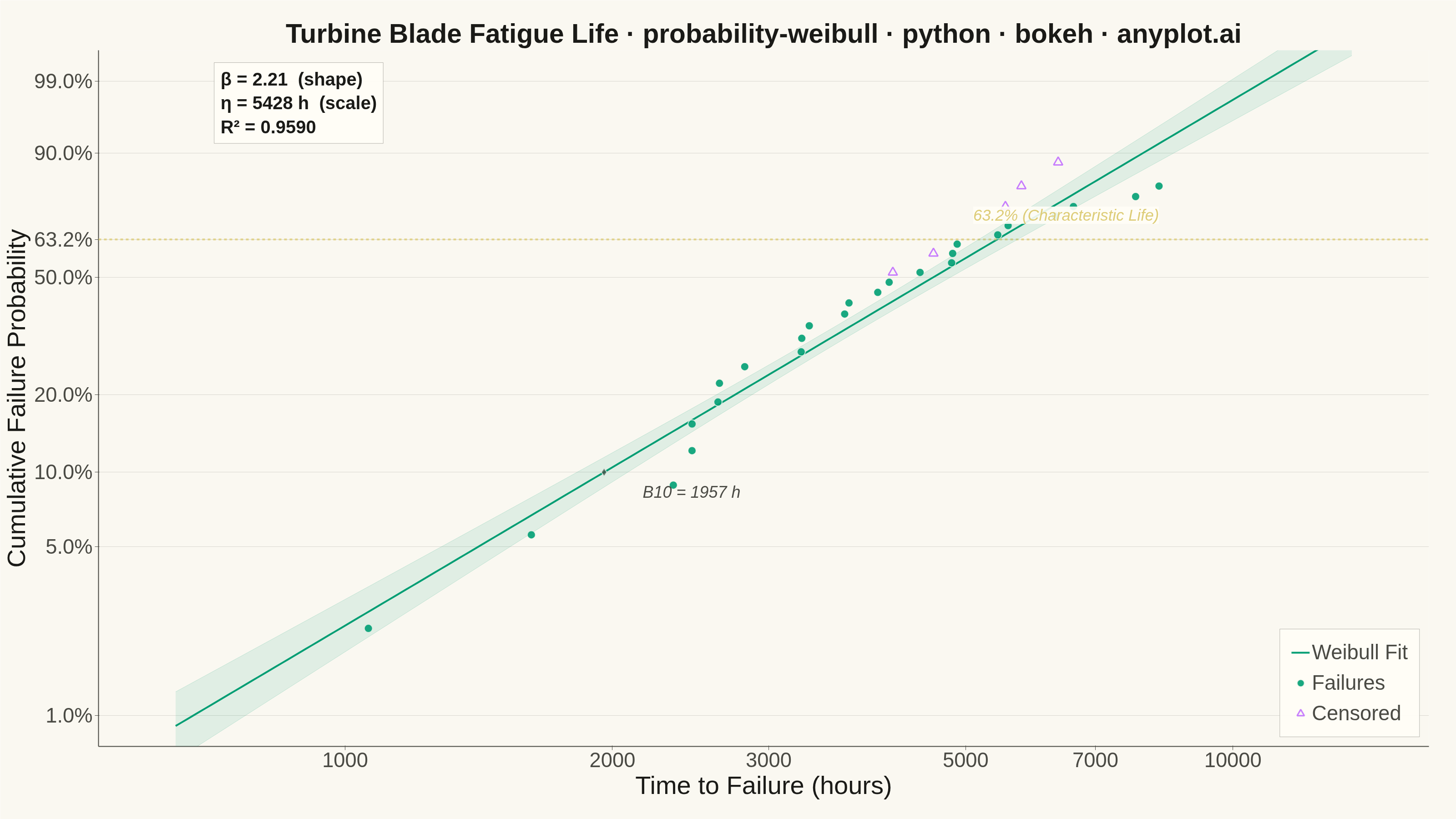
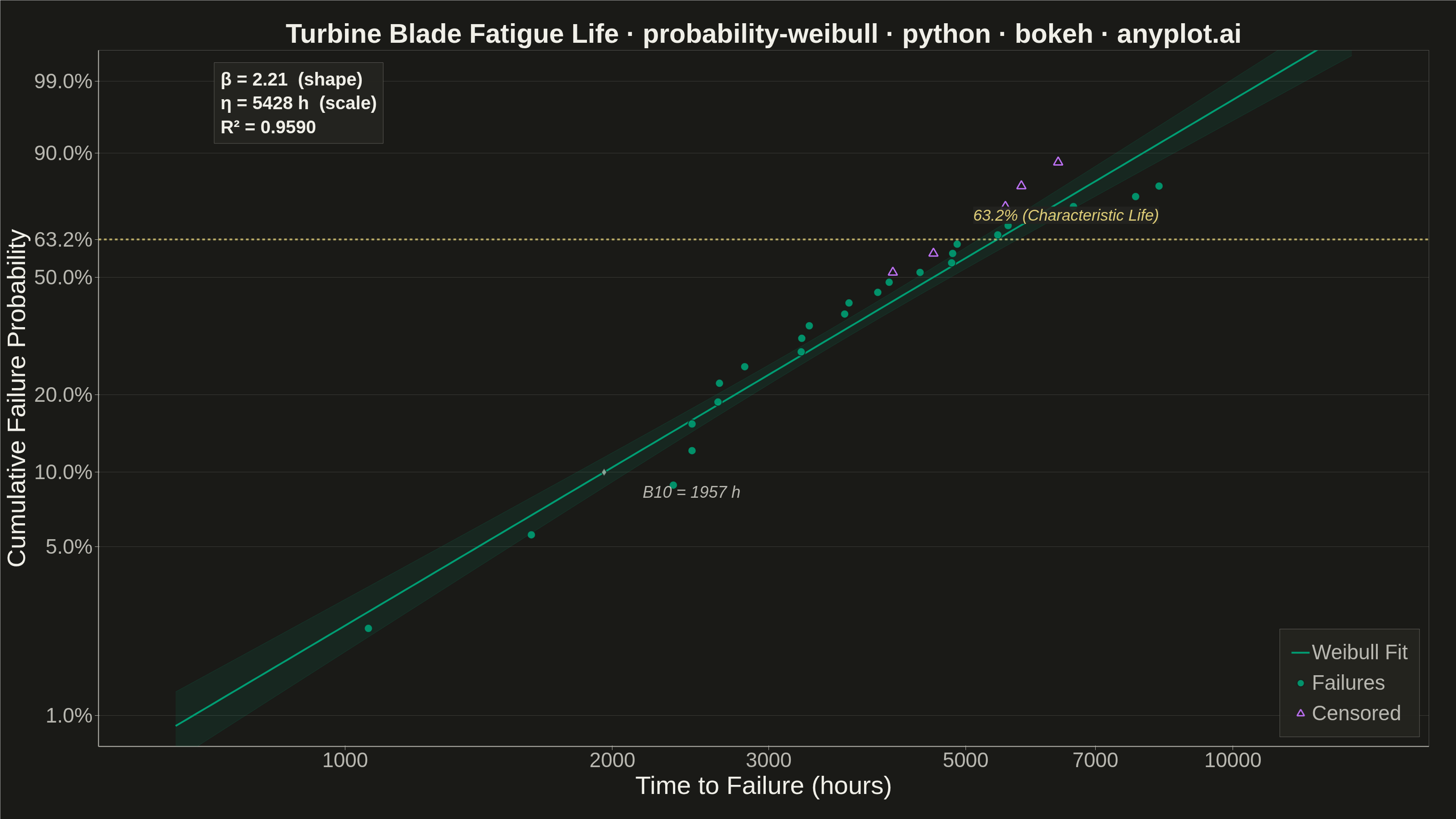
A Weibull probability plot displays failure or lifetime data on Weibull probability paper (logarithmic x-axis for time/cycles, linearized Weibull CDF on y-axis) with a fitted straight line. It is the standard tool in reliability engineering for estimating Weibull distribution parameters (shape and scale), assessing whether data follow a Weibull distribution, and extrapolating failure probabilities. The slope of the fitted line gives the shape parameter (beta), while the characteristic life (eta) is read at the 63.2% failure probability crossing.
""" anyplot.ai
probability-weibull: Weibull Probability Plot for Reliability Analysis
Library: bokeh 3.9.1 | Python 3.13.13
Quality: 93/100 | Updated: 2026-06-07
"""

import os
import sys
import time
from pathlib import Path


# bokeh.py is the script name — remove its directory from sys.path so that
# `import bokeh` resolves to the installed package, not this file itself.
_here = os.path.dirname(os.path.abspath(__file__))
sys.path[:] = [p for p in sys.path if os.path.abspath(p) != _here]

import numpy as np
from bokeh.io import output_file, save
from bokeh.models import Band, ColumnDataSource, HoverTool, Label, Span
from bokeh.plotting import figure
from scipy import stats
from selenium import webdriver
from selenium.webdriver.chrome.options import Options


# Theme-adaptive chrome tokens (Imprint palette)
THEME = os.getenv("ANYPLOT_THEME", "light")
PAGE_BG = "#FAF8F1" if THEME == "light" else "#1A1A17"
ELEVATED_BG = "#FFFDF6" if THEME == "light" else "#242420"
INK = "#1A1A17" if THEME == "light" else "#F0EFE8"
INK_SOFT = "#4A4A44" if THEME == "light" else "#B8B7B0"
INK_MUTED = "#6B6A63" if THEME == "light" else "#A8A79F"

# Imprint palette
BRAND = "#009E73"  # position 1 — failures (primary data)
LAVENDER = "#C475FD"  # position 2 — censored observations
ANYPLOT_AMBER = "#DDCC77"  # reference / caution line

# Data - Turbine blade fatigue-life data (hours to failure)
np.random.seed(42)
n_failures = 25
n_censored = 5
n_total = n_failures + n_censored

# Generate Weibull-distributed failure times (shape=2.5, scale=5000)
true_beta = 2.5
true_eta = 5000
failure_times = np.sort(stats.weibull_min.rvs(true_beta, scale=true_eta, size=n_failures))

# Censored observations (suspended tests, typically at higher times)
censored_times = np.sort(np.random.uniform(4000, 7000, size=n_censored))

# Combine and compute median rank plotting positions for failures only
# Using Bernard's approximation: (i - 0.3) / (n + 0.4)
ranks = np.arange(1, n_failures + 1)
median_rank = (ranks - 0.3) / (n_total + 0.4)

# Weibull linearized y-axis: ln(-ln(1 - F))
weibull_y = np.log(-np.log(1 - median_rank))
log_failure_times = np.log(failure_times)

# Fit line in linearized space: weibull_y = beta * ln(t) - beta * ln(eta)
slope_fit, intercept_fit, r_value, _, _ = stats.linregress(log_failure_times, weibull_y)
beta_fit = slope_fit
eta_fit = np.exp(-intercept_fit / beta_fit)
r_squared = r_value**2

# Fitted line data
log_t_line = np.linspace(np.log(failure_times.min()) - 0.5, np.log(failure_times.max()) + 0.5, 200)
weibull_y_line = beta_fit * log_t_line - beta_fit * np.log(eta_fit)

# Reference probability levels for y-axis labels
prob_levels = np.array([0.01, 0.05, 0.10, 0.20, 0.50, 0.632, 0.90, 0.99])
weibull_y_levels = np.log(-np.log(1 - prob_levels))

# B10 life calculation (10% failure probability)
b10_weibull_y = np.log(-np.log(1 - 0.10))
b10_life = eta_fit * (-np.log(1 - 0.10)) ** (1 / beta_fit)

# 63.2% characteristic life reference
char_life_y = np.log(-np.log(1 - 0.632))

# Compute censored plotting positions using adjusted ranks
all_times = np.concatenate([failure_times, censored_times])
all_censored = np.concatenate([np.zeros(n_failures), np.ones(n_censored)])
sort_idx = np.argsort(all_times)
all_times_sorted = all_times[sort_idx]
all_censored_sorted = all_censored[sort_idx]

reverse_ranks = np.arange(n_total, 0, -1)
adjusted_rank = np.zeros(n_total)
prev_adj = 0
for i in range(n_total):
    if all_censored_sorted[i] == 0:
        prev_adj += 1
        adjusted_rank[i] = prev_adj
    else:
        increment = (n_total + 1 - prev_adj) / (reverse_ranks[i] + 1)
        prev_adj += increment
        adjusted_rank[i] = prev_adj

censored_mask = all_censored_sorted == 1
censored_adjusted_ranks = adjusted_rank[censored_mask]
censored_median_rank = (censored_adjusted_ranks - 0.3) / (n_total + 0.4)
censored_median_rank = np.clip(censored_median_rank, 0.001, 0.999)
censored_weibull_y = np.log(-np.log(1 - censored_median_rank))

# Data sources
failure_source = ColumnDataSource(
    data={
        "time": failure_times,
        "log_time": log_failure_times,
        "weibull_y": weibull_y,
        "prob_pct": [f"{p * 100:.1f}%" for p in median_rank],
        "time_fmt": [f"{t:.0f}" for t in failure_times],
    }
)

censored_source = ColumnDataSource(
    data={
        "time": censored_times,
        "log_time": np.log(censored_times),
        "weibull_y": censored_weibull_y,
        "time_fmt": [f"{t:.0f}" for t in censored_times],
    }
)

# Confidence band (approximate ±2 SE)
se_y = np.sqrt(
    (1 - r_squared)
    * np.var(weibull_y)
    * (
        1 / len(weibull_y)
        + (log_t_line - np.mean(log_failure_times)) ** 2 / np.sum((log_failure_times - np.mean(log_failure_times)) ** 2)
    )
)
band_source = ColumnDataSource(
    data={
        "log_time": log_t_line,
        "weibull_y": weibull_y_line,
        "upper": weibull_y_line + 2 * se_y,
        "lower": weibull_y_line - 2 * se_y,
    }
)
line_source = ColumnDataSource(data={"log_time": log_t_line, "weibull_y": weibull_y_line})

# Title — descriptive prefix + spec-id · language · library · anyplot.ai
# "Turbine Blade Fatigue Life · probability-weibull · python · bokeh · anyplot.ai" = 76 chars
# fontsize = round(50 * 67 / 76) = 44pt
TITLE = "Turbine Blade Fatigue Life · probability-weibull · python · bokeh · anyplot.ai"

# Canvas: 3200×1800 (landscape 16:9) per bokeh.md hard rule
W, H = 3200, 1800
p = figure(
    width=W,
    height=H,
    title=TITLE,
    x_axis_label="Time to Failure (hours)",
    y_axis_label="Cumulative Failure Probability",
    x_range=(log_t_line.min() - 0.2, log_t_line.max() + 0.2),
    y_range=(weibull_y_levels[0] - 0.3, weibull_y_levels[-1] + 0.3),
    toolbar_location=None,
    min_border_bottom=160,
    min_border_left=200,
    min_border_top=110,
    min_border_right=60,
)

# Theme-adaptive backgrounds
p.background_fill_color = PAGE_BG
p.border_fill_color = PAGE_BG
p.outline_line_color = INK_SOFT

# 63.2% characteristic life reference line
char_life_span = Span(
    location=char_life_y, dimension="width", line_color=ANYPLOT_AMBER, line_width=4, line_dash="dashed", line_alpha=0.8
)
p.add_layout(char_life_span)

# 95% confidence band
band = Band(
    base="log_time",
    lower="lower",
    upper="upper",
    source=band_source,
    fill_color=BRAND,
    fill_alpha=0.1,
    line_color=BRAND,
    line_alpha=0.2,
    line_width=1,
)
p.add_layout(band)

# Fitted line
p.line("log_time", "weibull_y", source=line_source, line_color=BRAND, line_width=4, legend_label="Weibull Fit")

# Failure data points (filled circles)
failure_renderer = p.scatter(
    "log_time",
    "weibull_y",
    source=failure_source,
    size=18,
    color=BRAND,
    alpha=0.9,
    line_color=PAGE_BG,
    line_width=2,
    legend_label="Failures",
)

# Censored data points (hollow triangles — distinct shape from failures)
censored_renderer = p.scatter(
    "log_time",
    "weibull_y",
    source=censored_source,
    size=20,
    marker="triangle",
    color=PAGE_BG,
    alpha=0.95,
    line_color=LAVENDER,
    line_width=3,
    legend_label="Censored",
)

# Hover tools
hover_failure = HoverTool(
    renderers=[failure_renderer],
    tooltips=[("Time", "@time_fmt hours"), ("Cum. Probability", "@prob_pct")],
    mode="mouse",
)
p.add_tools(hover_failure)

hover_censored = HoverTool(renderers=[censored_renderer], tooltips=[("Censored at", "@time_fmt hours")], mode="mouse")
p.add_tools(hover_censored)

# Parameter annotation box — placed below the top tick so text flows downward fully visible
param_text = f"β = {beta_fit:.2f}  (shape)\nη = {eta_fit:.0f} h  (scale)\nR² = {r_squared:.4f}"
param_label = Label(
    x=log_t_line.min() + 0.1,
    y=weibull_y_levels[-1] - 0.6,
    text=param_text,
    text_font_size="30pt",
    text_color=INK,
    text_font_style="bold",
    background_fill_color=ELEVATED_BG,
    background_fill_alpha=0.95,
    border_line_color=INK_SOFT,
    border_line_alpha=0.4,
    padding=14,
)
p.add_layout(param_label)

# 63.2% characteristic life label
char_label = Label(
    x=log_t_line.max() - 0.5,
    y=char_life_y + 0.15,
    text="63.2% (Characteristic Life)",
    text_font_size="26pt",
    text_color=ANYPLOT_AMBER,
    text_font_style="italic",
    text_align="right",
    background_fill_color=ELEVATED_BG,
    background_fill_alpha=0.9,
)
p.add_layout(char_label)

# B10 life annotation (10% failure probability)
b10_label = Label(
    x=np.log(b10_life) + 0.1,
    y=b10_weibull_y - 0.28,
    text=f"B10 = {b10_life:.0f} h",
    text_font_size="27pt",
    text_color=INK_SOFT,
    text_font_style="italic",
)
p.add_layout(b10_label)

# B10 reference marker on the fit line
p.scatter(
    [np.log(b10_life)],
    [b10_weibull_y],
    size=18,
    marker="diamond",
    color=INK_SOFT,
    alpha=0.8,
    line_color=PAGE_BG,
    line_width=2,
)

# Custom y-axis tick labels showing probability percentages
p.yaxis.ticker = list(weibull_y_levels)
prob_labels = {float(y): f"{p * 100:.1f}%" for y, p in zip(weibull_y_levels, prob_levels, strict=True)}
p.yaxis.major_label_overrides = prob_labels

# Custom x-axis: show actual hours
log_tick_values = np.log([1000, 2000, 3000, 5000, 7000, 10000])
p.xaxis.ticker = list(log_tick_values)
time_labels = {float(lt): f"{np.exp(lt):.0f}" for lt in log_tick_values}
p.xaxis.major_label_overrides = time_labels

# Title
p.title.text_font_size = "44pt"
p.title.text_color = INK
p.title.align = "center"

# Axis labels and ticks
p.xaxis.axis_label_text_font_size = "42pt"
p.yaxis.axis_label_text_font_size = "42pt"
p.xaxis.axis_label_text_color = INK
p.yaxis.axis_label_text_color = INK
p.xaxis.axis_label_text_font_style = "normal"
p.yaxis.axis_label_text_font_style = "normal"
p.xaxis.major_label_text_font_size = "34pt"
p.yaxis.major_label_text_font_size = "34pt"
p.xaxis.major_label_text_color = INK_SOFT
p.yaxis.major_label_text_color = INK_SOFT

# Legend
p.legend.label_text_font_size = "34pt"
p.legend.label_text_color = INK_SOFT
p.legend.location = "bottom_right"
p.legend.background_fill_color = ELEVATED_BG
p.legend.background_fill_alpha = 0.92
p.legend.border_line_color = INK_SOFT
p.legend.border_line_alpha = 0.4
p.legend.glyph_height = 40
p.legend.glyph_width = 40
p.legend.padding = 25
p.legend.spacing = 15
p.legend.margin = 20

# Grid — minimal y-grid only for Weibull paper look
p.xgrid.grid_line_color = None
p.ygrid.grid_line_color = INK
p.ygrid.grid_line_alpha = 0.15

# Axes chrome
p.xaxis.axis_line_color = INK_SOFT
p.yaxis.axis_line_color = INK_SOFT
p.xaxis.axis_line_width = 2
p.yaxis.axis_line_width = 2
p.xaxis.minor_tick_line_color = None
p.yaxis.minor_tick_line_color = None
p.xaxis.major_tick_line_color = INK_SOFT
p.yaxis.major_tick_line_color = INK_SOFT
p.xaxis.major_tick_out = 8
p.yaxis.major_tick_out = 8

p.outline_line_color = None

# Save HTML (interactive artifact)
output_file(f"plot-{THEME}.html")
save(p)

# Screenshot with headless Chrome (Selenium 4 / Selenium Manager)
# Use CDP setDeviceMetricsOverride so the inner viewport is authoritative:
# --window-size alone is eaten by Chrome in headless mode (gives 1661 instead of 1800).
opts = Options()
for arg in (
    "--headless=new",
    "--no-sandbox",
    "--disable-dev-shm-usage",
    "--disable-gpu",
    f"--window-size={W},{H}",
    "--hide-scrollbars",
):
    opts.add_argument(arg)
driver = webdriver.Chrome(options=opts)
driver.execute_cdp_cmd(
    "Emulation.setDeviceMetricsOverride", {"width": W, "height": H, "deviceScaleFactor": 1, "mobile": False}
)
driver.get(f"file://{Path(f'plot-{THEME}.html').resolve()}")
time.sleep(3)
driver.save_screenshot(f"plot-{THEME}.png")
driver.quit()

# Pin to exact canvas dims so the post-render gate passes
from PIL import Image as _PILImage


_img = _PILImage.open(f"plot-{THEME}.png").convert("RGB")
if _img.size != (W, H):
    _norm = _PILImage.new("RGB", (W, H), PAGE_BG)
    _norm.paste(_img, ((W - _img.size[0]) // 2, (H - _img.size[1]) // 2))
    _norm.save(f"plot-{THEME}.png")
Runnable source as JSON, for any HTTP client: https://api.anyplot.ai/specs/probability-weibull/bokeh/code. Any spec id and library id listed in llms-full.txt fit the same URL shape; every URL below is complete and callable.
{
  "spec_id": "probability-weibull",
  "language": "python",
  "library": "bokeh",
  "page": "https://anyplot.ai/probability-weibull/python/bokeh",
  "hub": "https://anyplot.ai/probability-weibull",
  "code_json": "https://api.anyplot.ai/specs/probability-weibull/bokeh/code",
  "spec_json": "https://api.anyplot.ai/specs/probability-weibull",
  "render_light_png": "https://storage.googleapis.com/anyplot-images/plots/probability-weibull/python/bokeh/plot-light.png",
  "render_dark_png": "https://storage.googleapis.com/anyplot-images/plots/probability-weibull/python/bokeh/plot-dark.png",
  "interactive_light_html": "https://storage.googleapis.com/anyplot-images/plots/probability-weibull/python/bokeh/plot-light.html",
  "interactive_dark_html": "https://storage.googleapis.com/anyplot-images/plots/probability-weibull/python/bokeh/plot-dark.html",
  "quality_score": 93.0,
  "license": "MIT",
  "guide": "https://anyplot.ai/llms.txt"
}
Part of Weibull Probability Plot for Reliability Analysis on anyplot.ai.