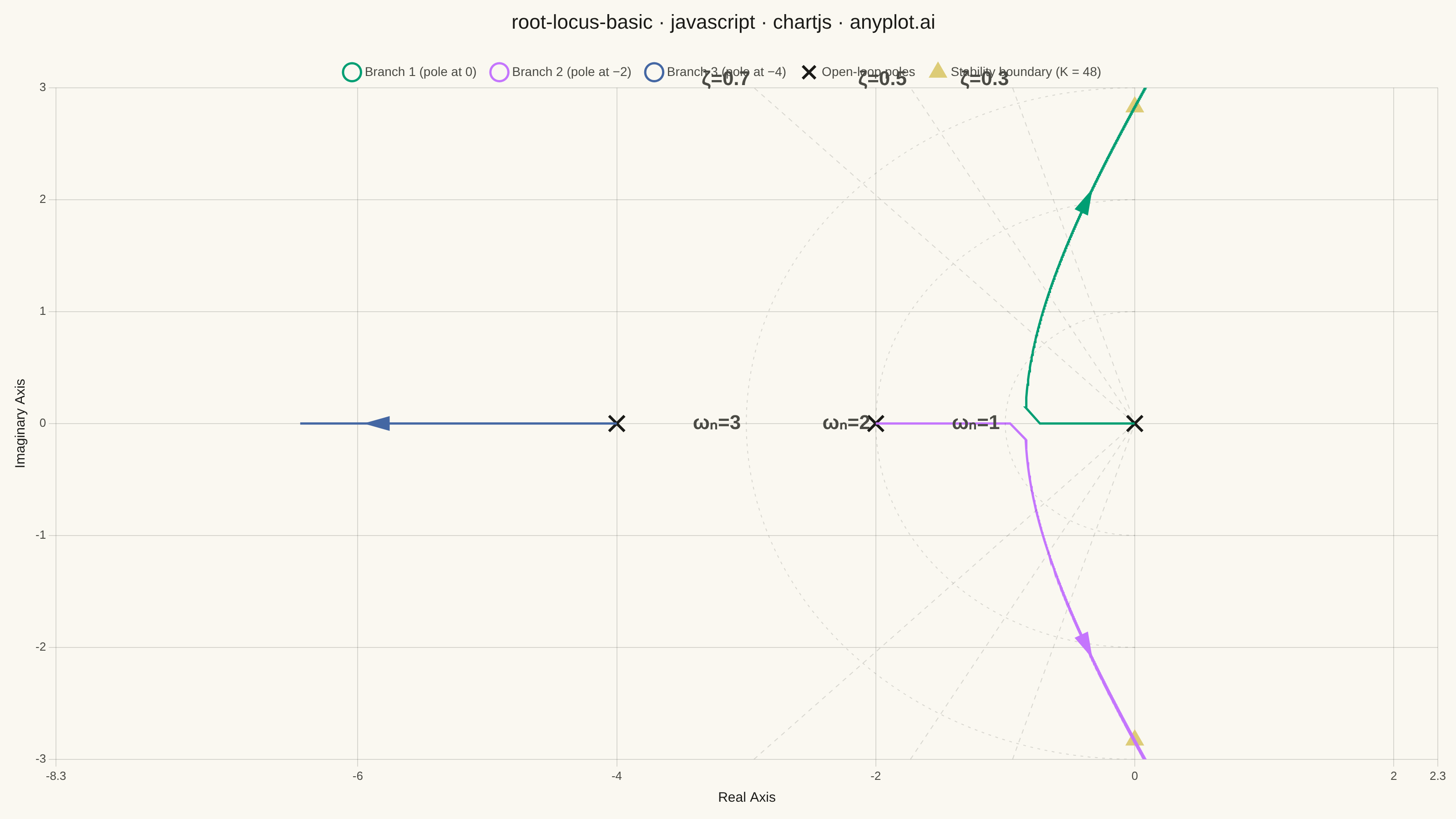
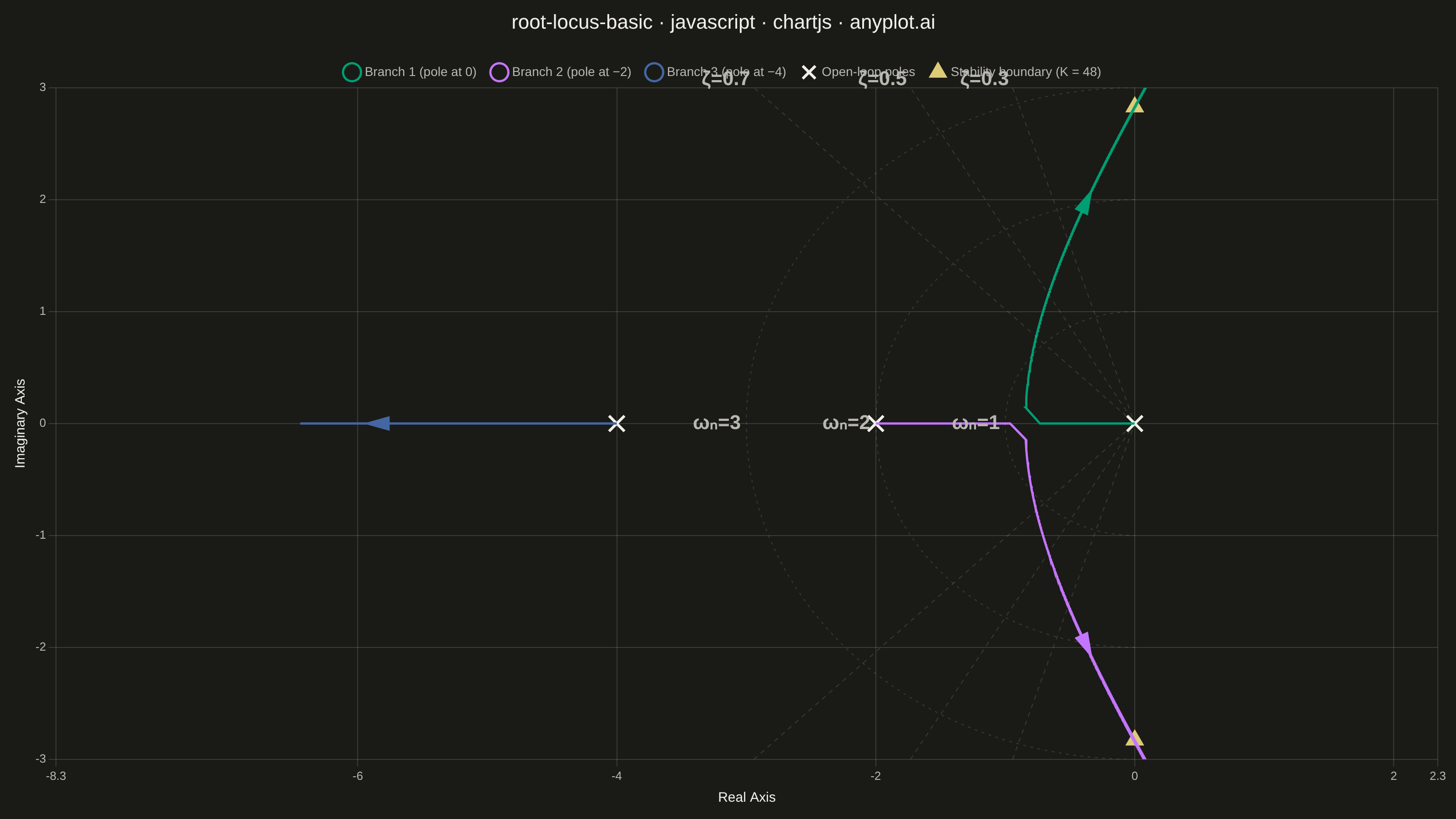
A root locus plot traces how the closed-loop poles of a transfer function migrate through the complex plane as a system parameter (typically gain K) varies from 0 to infinity. It is a fundamental tool in classical control theory for analyzing system stability and designing controllers. The plot reveals critical information about pole trajectories, stability boundaries, and gain margins.
// anyplot.ai
// root-locus-basic: Root Locus Plot for Control Systems
// Library: chartjs 4.4.7 | JavaScript 22.22.3
// Quality: 86/100 | Created: 2026-06-18

//# anyplot-orientation: landscape
const t = window.ANYPLOT_TOKENS;

// Horner evaluation of monic cubic s³ + p·s² + q·s + r at complex z = (zr + j·zi)
function evalCubic(p, q, r, zr, zi) {
  let re = 1, im = 0;
  for (const c of [p, q, r]) {
    const nr = re * zr - im * zi + c;
    const ni = re * zi + im * zr;
    re = nr; im = ni;
  }
  return { re, im };
}

// Durand–Kerner method: three roots of s³ + p·s² + q·s + r = 0
function cubicRoots(p, q, r) {
  let z = [{ re: 0.5, im: 0.6 }, { re: -0.7, im: 0.3 }, { re: 0.2, im: -0.8 }];
  for (let it = 0; it < 150; it++) {
    for (let i = 0; i < 3; i++) {
      const f = evalCubic(p, q, r, z[i].re, z[i].im);
      let dr = 1, di = 0;
      for (let j = 0; j < 3; j++) {
        if (j === i) continue;
        const nr = dr * (z[i].re - z[j].re) - di * (z[i].im - z[j].im);
        const ni = dr * (z[i].im - z[j].im) + di * (z[i].re - z[j].re);
        dr = nr; di = ni;
      }
      const d2 = dr * dr + di * di;
      if (d2 < 1e-28) continue;
      z[i].re -= (f.re * dr + f.im * di) / d2;
      z[i].im -= (f.im * dr - f.re * di) / d2;
    }
  }
  return z.sort((a, b) =>
    Math.abs(a.re - b.re) > 0.01 ? b.re - a.re : b.im - a.im
  );
}

// G(s) = K / [s(s+2)(s+4)]  →  s³ + 6s² + 8s + K = 0
// Poles: 0, −2, −4 | Breakaway ≈ −0.845 (K≈3.08) | Im-axis ±j√8 ≈ ±j2.83 (K=48)
const N = 600;
const K_MAX = 70;
const branches = [[], [], []];
for (let i = 0; i <= N; i++) {
  const K = (i / N) * K_MAX;
  const roots = cubicRoots(6, 8, K);
  for (let b = 0; b < 3; b++) {
    branches[b].push({ x: roots[b].re, y: roots[b].im });
  }
}

const openLoopPoles = [{ x: 0, y: 0 }, { x: -2, y: 0 }, { x: -4, y: 0 }];
const stabMarkers = [{ x: 0, y: Math.sqrt(8) }, { x: 0, y: -Math.sqrt(8) }];

// Equal pixel-per-unit scaling: canvas 3200×1800 → aspect 16:9
// X span 10.67 units, Y span 6.0 units → 300 px/unit each
const X_MIN = -8.33, X_MAX = 2.34, Y_MIN = -3.0, Y_MAX = 3.0;

// Constant-ζ reference lines (radial rays from origin into left half-plane)
// Slope: ω / |σ| = sqrt(1−ζ²) / ζ
const zetaDatasets = [0.3, 0.5, 0.7].map((zeta) => {
  const slope = Math.sqrt(1 - zeta * zeta) / zeta;
  // Clamp ray to Y boundary (Y_MAX / slope gives |σ| where ω hits Y_MAX)
  const sigmaEnd = Math.max(X_MIN, -Y_MAX / slope);
  const omegaEnd = Math.abs(sigmaEnd) * slope;
  return {
    label: `ζ = ${zeta}`,
    data: [{ x: sigmaEnd, y: -omegaEnd }, { x: 0, y: 0 }, { x: sigmaEnd, y: omegaEnd }],
    borderColor: t.grid,
    backgroundColor: "transparent",
    showLine: true,
    borderWidth: 1,
    borderDash: [5, 5],
    pointRadius: 0,
    tension: 0,
  };
});

// Constant-ωn reference arcs (left half-plane semicircles)
const omegaNDatasets = [1, 2, 3].map((wn) => {
  const pts = [];
  for (let i = 0; i <= 80; i++) {
    const angle = Math.PI / 2 + (Math.PI * i) / 80;
    pts.push({ x: wn * Math.cos(angle), y: wn * Math.sin(angle) });
  }
  return {
    label: `ωₙ = ${wn}`,
    data: pts,
    borderColor: t.grid,
    backgroundColor: "transparent",
    showLine: true,
    borderWidth: 1,
    borderDash: [3, 5],
    pointRadius: 0,
    tension: 0,
  };
});

const canvas = document.createElement("canvas");
document.getElementById("container").appendChild(canvas);

const title = "root-locus-basic · javascript · chartjs · anyplot.ai";
const titleSize = title.length > 67 ? Math.round(22 * 67 / title.length) : 22;

new Chart(canvas, {
  type: "scatter",
  data: {
    datasets: [
      // Reference overlays drawn first (behind branches)
      ...zetaDatasets,
      ...omegaNDatasets,
      // Locus branches
      {
        label: "Branch 1 (pole at 0)",
        data: branches[0],
        borderColor: t.palette[0],
        backgroundColor: "transparent",
        showLine: true,
        borderWidth: 2.5,
        pointRadius: 0,
        tension: 0,
      },
      {
        label: "Branch 2 (pole at −2)",
        data: branches[1],
        borderColor: t.palette[1],
        backgroundColor: "transparent",
        showLine: true,
        borderWidth: 2.5,
        pointRadius: 0,
        tension: 0,
      },
      {
        label: "Branch 3 (pole at −4)",
        data: branches[2],
        borderColor: t.palette[2],
        backgroundColor: "transparent",
        showLine: true,
        borderWidth: 2.5,
        pointRadius: 0,
        tension: 0,
      },
      // Landmarks
      {
        label: "Open-loop poles",
        data: openLoopPoles,
        borderColor: t.ink,
        backgroundColor: "transparent",
        pointStyle: "crossRot",
        pointRadius: 12,
        pointBorderWidth: 3,
        showLine: false,
      },
      {
        label: "Stability boundary (K = 48)",
        data: stabMarkers,
        borderColor: t.amber,
        backgroundColor: t.amber,
        pointStyle: "triangle",
        pointRadius: 10,
        pointBorderWidth: 2,
        showLine: false,
      },
    ],
  },
  plugins: [
    {
      id: "bg",
      beforeDraw: (chart) => {
        const ctx = chart.ctx;
        ctx.save();
        ctx.fillStyle = t.pageBg;
        ctx.fillRect(0, 0, chart.width, chart.height);
        ctx.restore();
      },
    },
    {
      // Gain-direction arrows: filled triangles at branch midpoints
      id: "gainArrows",
      afterDatasetsDraw: (chart) => {
        const ctx = chart.ctx;
        const xs = chart.scales.x;
        const ys = chart.scales.y;
        const arrowSpec = [
          { branch: branches[0], color: t.palette[0], midIdx: 180 },
          { branch: branches[1], color: t.palette[1], midIdx: 180 },
          { branch: branches[2], color: t.palette[2], midIdx: 350 },
        ];
        for (const { branch, color, midIdx } of arrowSpec) {
          const p0 = branch[midIdx];
          const p1 = branch[Math.min(midIdx + 10, branch.length - 1)];
          const x0 = xs.getPixelForValue(p0.x);
          const y0 = ys.getPixelForValue(p0.y);
          const x1 = xs.getPixelForValue(p1.x);
          const y1 = ys.getPixelForValue(p1.y);
          const angle = Math.atan2(y1 - y0, x1 - x0);
          const sz = 18;
          ctx.save();
          ctx.translate(x0, y0);
          ctx.rotate(angle);
          ctx.fillStyle = color;
          ctx.beginPath();
          ctx.moveTo(sz, 0);
          ctx.lineTo(-sz * 0.6, sz * 0.45);
          ctx.lineTo(-sz * 0.6, -sz * 0.45);
          ctx.closePath();
          ctx.fill();
          ctx.restore();
        }
      },
    },
    {
      // Label ζ and ωn reference lines directly on the chart
      id: "refLabels",
      afterDatasetsDraw: (chart) => {
        const ctx = chart.ctx;
        const xs = chart.scales.x;
        const ys = chart.scales.y;
        ctx.save();
        ctx.font = "600 22px sans-serif";
        ctx.fillStyle = t.inkSoft;
        ctx.textAlign = "right";
        ctx.textBaseline = "bottom";
        // ζ labels at upper ray endpoints
        [0.3, 0.5, 0.7].forEach((zeta) => {
          const slope = Math.sqrt(1 - zeta * zeta) / zeta;
          const sigmaEnd = Math.max(X_MIN, -Y_MAX / slope);
          const omegaEnd = Math.abs(sigmaEnd) * slope;
          const px = xs.getPixelForValue(sigmaEnd) - 4;
          const py = ys.getPixelForValue(omegaEnd) + 2;
          ctx.fillText(`ζ=${zeta}`, px, py);
        });
        // ωn labels at leftmost arc point (angle = π)
        ctx.textAlign = "right";
        ctx.textBaseline = "middle";
        [1, 2, 3].forEach((wn) => {
          const px = xs.getPixelForValue(-wn) - 6;
          const py = ys.getPixelForValue(0);
          ctx.fillText(`ωₙ=${wn}`, px, py);
        });
        ctx.restore();
      },
    },
  ],
  options: {
    responsive: true,
    maintainAspectRatio: false,
    animation: false,
    layout: { padding: { top: 4, right: 20, bottom: 10, left: 10 } },
    plugins: {
      title: {
        display: true,
        text: title,
        color: t.ink,
        font: { size: titleSize, weight: "500" },
        padding: { top: 8, bottom: 16 },
      },
      legend: {
        labels: {
          color: t.inkSoft,
          font: { size: 14 },
          usePointStyle: true,
          padding: 18,
          // Exclude reference overlay datasets from legend
          filter: (item) => !item.text.startsWith("ζ") && !item.text.startsWith("ω"),
        },
      },
    },
    scales: {
      x: {
        type: "linear",
        min: X_MIN,
        max: X_MAX,
        ticks: { color: t.inkSoft, font: { size: 13 } },
        grid: { color: t.grid },
        border: { display: false },
        title: {
          display: true,
          text: "Real Axis",
          color: t.ink,
          font: { size: 15, weight: "500" },
        },
      },
      y: {
        type: "linear",
        min: Y_MIN,
        max: Y_MAX,
        ticks: { color: t.inkSoft, font: { size: 13 } },
        grid: { color: t.grid },
        border: { display: false },
        title: {
          display: true,
          text: "Imaginary Axis",
          color: t.ink,
          font: { size: 15, weight: "500" },
        },
      },
    },
  },
});
Runnable source as JSON, for any HTTP client: https://api.anyplot.ai/specs/root-locus-basic/chartjs/code. Any spec id and library id listed in llms-full.txt fit the same URL shape; every URL below is complete and callable.
{
  "spec_id": "root-locus-basic",
  "language": "javascript",
  "library": "chartjs",
  "page": "https://anyplot.ai/root-locus-basic/javascript/chartjs",
  "hub": "https://anyplot.ai/root-locus-basic",
  "code_json": "https://api.anyplot.ai/specs/root-locus-basic/chartjs/code",
  "spec_json": "https://api.anyplot.ai/specs/root-locus-basic",
  "render_light_png": "https://storage.googleapis.com/anyplot-images/plots/root-locus-basic/javascript/chartjs/plot-light.png",
  "render_dark_png": "https://storage.googleapis.com/anyplot-images/plots/root-locus-basic/javascript/chartjs/plot-dark.png",
  "interactive_light_html": "https://storage.googleapis.com/anyplot-images/plots/root-locus-basic/javascript/chartjs/plot-light.html",
  "interactive_dark_html": "https://storage.googleapis.com/anyplot-images/plots/root-locus-basic/javascript/chartjs/plot-dark.html",
  "quality_score": 86.0,
  "license": "MIT",
  "guide": "https://anyplot.ai/llms.txt"
}
Part of Root Locus Plot for Control Systems on anyplot.ai.