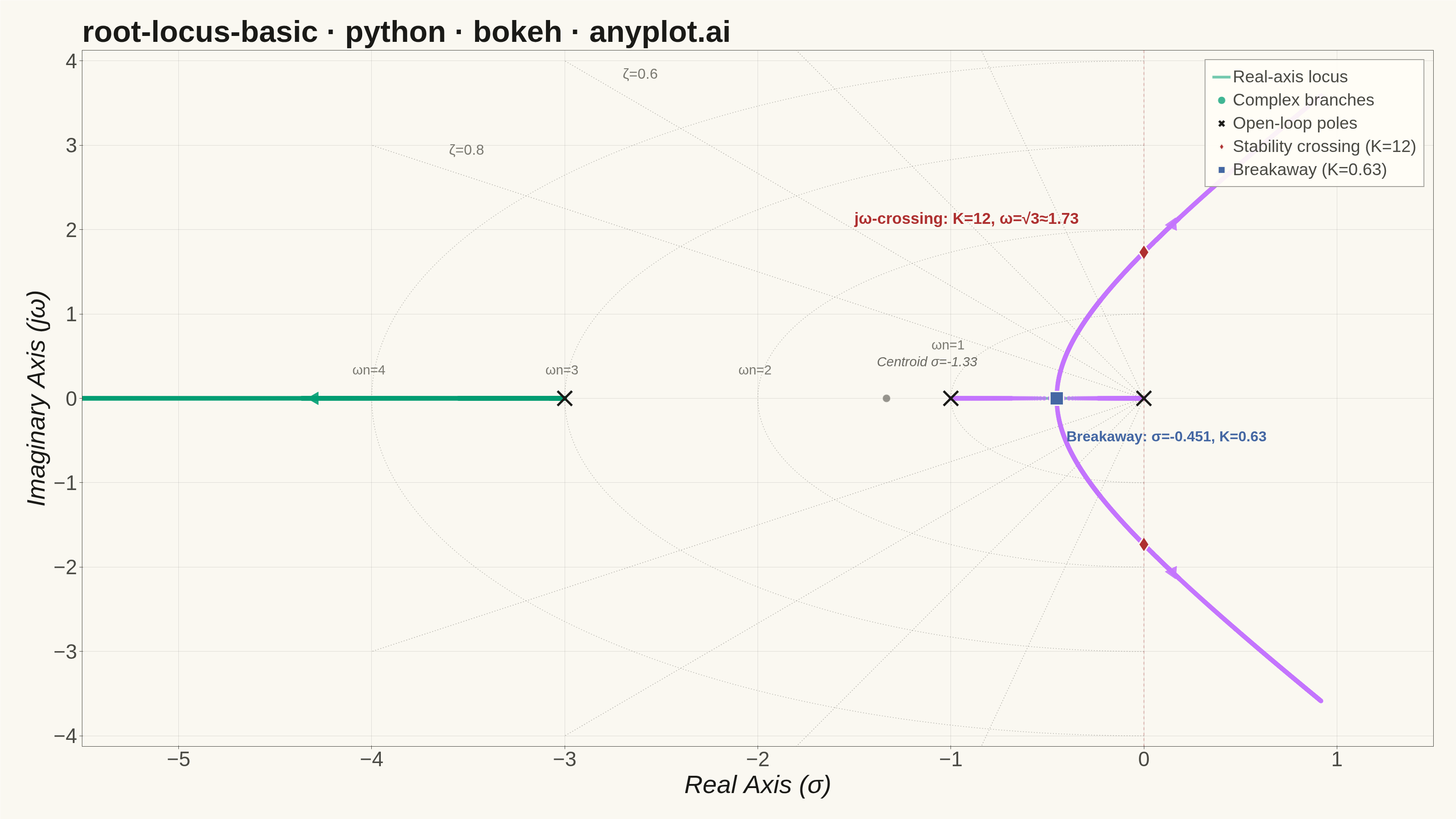
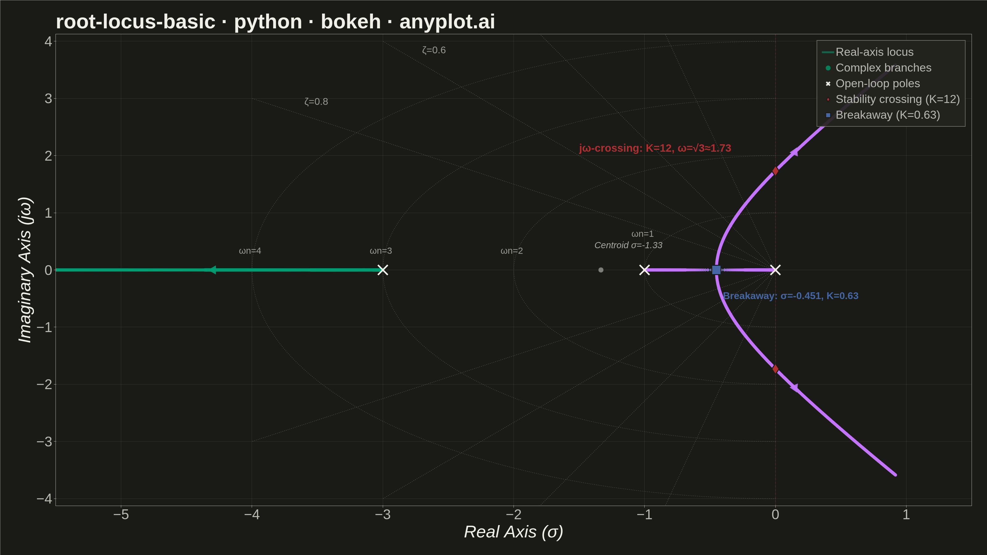
A root locus plot traces how the closed-loop poles of a transfer function migrate through the complex plane as a system parameter (typically gain K) varies from 0 to infinity. It is a fundamental tool in classical control theory for analyzing system stability and designing controllers. The plot reveals critical information about pole trajectories, stability boundaries, and gain margins.
""" anyplot.ai
root-locus-basic: Root Locus Plot for Control Systems
Library: bokeh 3.9.1 | Python 3.13.14
Quality: 89/100 | Updated: 2026-06-18
"""

# Remove the script's own directory from sys.path so that `import bokeh` resolves
# to the installed package rather than this file (which shares the name "bokeh.py").
import os as _os
import sys as _sys


_here = _os.path.dirname(_os.path.abspath(__file__))
_sys.path = [p for p in _sys.path if not p or _os.path.abspath(p) != _here]
del _sys, _os, _here

import os
import time
from pathlib import Path

import numpy as np
from bokeh.io import output_file, save
from bokeh.models import ColumnDataSource, HoverTool, Label, Range1d, Span
from bokeh.plotting import figure
from selenium import webdriver
from selenium.webdriver.chrome.options import Options


# Theme tokens (Imprint palette — theme-adaptive chrome)
THEME = os.getenv("ANYPLOT_THEME", "light")
PAGE_BG = "#FAF8F1" if THEME == "light" else "#1A1A17"
ELEVATED_BG = "#FFFDF6" if THEME == "light" else "#242420"
INK = "#1A1A17" if THEME == "light" else "#F0EFE8"
INK_SOFT = "#4A4A44" if THEME == "light" else "#B8B7B0"
INK_MUTED = "#6B6A63" if THEME == "light" else "#A8A79F"

# Imprint categorical palette — hybrid-v3 sort order
BRAND = "#009E73"  # position 1 — branch 1 (real-axis locus)
LAVENDER = "#C475FD"  # position 2 — branches 2 & 3 (complex conjugate pair)
BLUE = "#4467A3"  # position 3 — breakaway annotation
MATTE_RED = "#AE3030"  # position 5 — stability boundary (semantic: error/bad)

# Data — Transfer function G(s) = 1 / (s(s+1)(s+3))
# Open-loop poles at s = 0, -1, -3; no zeros
open_loop_poles = np.array([0.0, -1.0, -3.0])

# Characteristic equation: s³ + 4s² + 3s + K = 0
gains = np.concatenate(
    [np.linspace(0, 0.5, 200), np.linspace(0.5, 5, 600), np.linspace(5, 20, 600), np.linspace(20, 80, 600)]
)

all_roots = np.zeros((len(gains), 3), dtype=complex)
for i, k in enumerate(gains):
    all_roots[i] = np.sort_complex(np.roots([1, 4, 3, k]))

# Organise into branches
n_branches = 3
branch_real, branch_imag, branch_gain, branch_id = [], [], [], []
branch_colors_map = [BRAND, LAVENDER, LAVENDER]

for b in range(n_branches):
    branch_real.extend(all_roots[:, b].real)
    branch_imag.extend(all_roots[:, b].imag)
    branch_gain.extend(gains)
    branch_id.extend([f"Branch {b + 1}"] * len(gains))

branch_real = np.array(branch_real)
branch_imag = np.array(branch_imag)
branch_gain = np.array(branch_gain)
colors = [c for b in range(n_branches) for c in [branch_colors_map[b]] * len(gains)]

source = ColumnDataSource(
    data={"real": branch_real, "imag": branch_imag, "gain": branch_gain, "branch": branch_id, "color": colors}
)
pole_source = ColumnDataSource(data={"real": open_loop_poles, "imag": np.zeros_like(open_loop_poles)})

# Key engineering values (Routh criterion for s³ + 4s² + 3s + K = 0)
w_crit = np.sqrt(3)
crossing_source = ColumnDataSource(data={"real": [0.0, 0.0], "imag": [w_crit, -w_crit]})

# Breakaway point: dK/ds = 0 → 3s² + 8s + 3 = 0
breakaway_s = (-8 + np.sqrt(28)) / 6
breakaway_K = -(breakaway_s**3 + 4 * breakaway_s**2 + 3 * breakaway_s)
centroid = open_loop_poles.sum() / len(open_loop_poles)

# Title — adaptive fontsize for longer strings (46 chars < 67 → default 50pt)
title = "root-locus-basic · python · bokeh · anyplot.ai"
n = len(title)
title_fontsize = f"{round(50 * 67 / n)}pt" if n > 67 else "50pt"

y_max = max(abs(branch_imag)) * 1.15

# Plot
p = figure(
    width=3200,
    height=1800,
    title=title,
    x_axis_label="Real Axis (σ)",
    y_axis_label="Imaginary Axis (jω)",
    x_range=Range1d(-5.5, 1.5),
    y_range=Range1d(-y_max, y_max),
    match_aspect=True,
    toolbar_location=None,  # prevents toolbar adding ~30-50px above canvas in PNG
    min_border_bottom=160,  # room for 34pt x-tick labels + 42pt x-axis label
    min_border_left=180,  # room for 34pt y-tick labels + 42pt y-axis label
    min_border_top=110,  # room for 50pt title
    min_border_right=50,
)

# Damping ratio guide lines — increased alpha (was 0.25, now 0.5) for better utility
for zeta in [0.2, 0.4, 0.6, 0.8]:
    r_max = 5.0
    x_end = -r_max * zeta
    y_end = r_max * np.sqrt(1 - zeta**2)
    p.line(x=[0, x_end], y=[0, y_end], line_color=INK_MUTED, line_width=1.5, line_alpha=0.5, line_dash="dotted")
    p.line(x=[0, x_end], y=[0, -y_end], line_color=INK_MUTED, line_width=1.5, line_alpha=0.5, line_dash="dotted")
    lx = -4.5 * zeta
    ly = 4.5 * np.sqrt(1 - zeta**2)
    p.add_layout(
        Label(x=lx, y=ly + 0.15, text=f"ζ={zeta}", text_font_size="24pt", text_color=INK_MUTED, text_alpha=0.9)
    )

# Natural frequency arcs — labels placed at arc midpoint to avoid legend overlap
for wn in [1, 2, 3, 4]:
    theta = np.linspace(np.pi / 2, np.pi, 60)
    arc_x = wn * np.cos(theta)
    arc_y = wn * np.sin(theta)
    p.line(
        x=arc_x.tolist(), y=arc_y.tolist(), line_color=INK_MUTED, line_width=1.5, line_alpha=0.45, line_dash="dotted"
    )
    p.line(
        x=arc_x.tolist(), y=(-arc_y).tolist(), line_color=INK_MUTED, line_width=1.5, line_alpha=0.45, line_dash="dotted"
    )
    # Label at leftmost point of arc; ωn=1 shifted up to avoid overlap with centroid annotation
    p.add_layout(
        Label(
            x=-wn - 0.1,
            y=(0.55 if wn == 1 else 0.25),
            text=f"ωn={wn}",
            text_font_size="22pt",
            text_color=INK_MUTED,
            text_alpha=0.9,
        )
    )

# Real-axis locus segments: [-1, 0] and (-∞, -3]
p.segment(
    x0=[-1], y0=[0], x1=[0], y1=[0], line_color=BRAND, line_width=6, line_alpha=0.55, legend_label="Real-axis locus"
)
p.segment(x0=[-5.5], y0=[0], x1=[-3], y1=[0], line_color=BRAND, line_width=6, line_alpha=0.55)

# Locus branches (size increased from 6 to 10 for better visibility)
scatter = p.scatter(
    x="real",
    y="imag",
    source=source,
    size=10,
    color="color",
    alpha=0.75,
    line_color=None,
    legend_label="Complex branches",
)

# Open-loop poles (× markers)
p.scatter(
    x="real", y="imag", source=pole_source, size=45, marker="x", color=INK, line_width=5, legend_label="Open-loop poles"
)

# Stability boundary crossings
p.scatter(
    x="real",
    y="imag",
    source=crossing_source,
    size=35,
    marker="diamond",
    color=MATTE_RED,
    line_color=PAGE_BG,
    line_width=3,
    legend_label="Stability crossing (K=12)",
)

# Breakaway point
p.scatter(
    x=[breakaway_s],
    y=[0],
    size=30,
    marker="square",
    color=BLUE,
    line_color=PAGE_BG,
    line_width=3,
    legend_label=f"Breakaway (K={breakaway_K:.2f})",
)

# Imaginary axis — stability boundary
p.add_layout(
    Span(location=0, dimension="height", line_color=MATTE_RED, line_width=2.5, line_alpha=0.25, line_dash="dashed")
)

# Direction arrows indicating increasing gain on each branch
for b in range(n_branches):
    arrow_idx = len(gains) * 2 // 3
    r = all_roots[arrow_idx, b]
    r_next = all_roots[min(arrow_idx + 20, len(gains) - 1), b]
    dx = r_next.real - r.real
    dy = r_next.imag - r.imag
    length = np.sqrt(dx**2 + dy**2)
    if length > 0.01:
        p.scatter(
            x=[r.real],
            y=[r.imag],
            size=28,
            marker="triangle",
            color=branch_colors_map[b],
            angle=[np.arctan2(dy, dx) - np.pi / 2],
            alpha=0.9,
        )

# Engineering annotations at key control theory points
p.add_layout(
    Label(
        x=-1.5,
        y=w_crit + 0.3,
        text=f"jω-crossing: K=12, ω=√3≈{w_crit:.2f}",
        text_font_size="26pt",
        text_color=MATTE_RED,
        text_font_style="bold",
    )
)

p.add_layout(
    Label(
        x=breakaway_s + 0.05,
        y=-0.55,
        text=f"Breakaway: σ={breakaway_s:.3f}, K={breakaway_K:.2f}",
        text_font_size="24pt",
        text_color=BLUE,
        text_font_style="bold",
    )
)

p.add_layout(
    Label(
        x=centroid - 0.05,
        y=0.35,
        text=f"Centroid σ={centroid:.2f}",
        text_font_size="22pt",
        text_color=INK_MUTED,
        text_font_style="italic",
    )
)
p.scatter(x=[centroid], y=[0], size=18, marker="circle", color=INK_MUTED, line_color=PAGE_BG, line_width=2, alpha=0.7)

# HoverTool (active in HTML preview)
p.add_tools(
    HoverTool(
        renderers=[scatter],
        tooltips=[("Pole", "@real{0.00} + @imag{0.00}j"), ("Gain K", "@gain{0.00}"), ("Branch", "@branch")],
        point_policy="snap_to_data",
        mode="mouse",
    )
)

# Theme-adaptive chrome
p.background_fill_color = PAGE_BG
p.border_fill_color = PAGE_BG
p.outline_line_color = INK_SOFT

p.title.text_font_size = title_fontsize
p.title.text_color = INK

p.xaxis.axis_label_text_font_size = "42pt"
p.yaxis.axis_label_text_font_size = "42pt"
p.xaxis.major_label_text_font_size = "34pt"
p.yaxis.major_label_text_font_size = "34pt"
p.xaxis.axis_label_text_color = INK
p.yaxis.axis_label_text_color = INK
p.xaxis.major_label_text_color = INK_SOFT
p.yaxis.major_label_text_color = INK_SOFT
p.xaxis.axis_line_color = INK_SOFT
p.yaxis.axis_line_color = INK_SOFT
p.xaxis.major_tick_line_color = INK_SOFT
p.yaxis.major_tick_line_color = INK_SOFT
p.xaxis.minor_tick_line_color = None
p.yaxis.minor_tick_line_color = None

p.xgrid.grid_line_color = INK
p.ygrid.grid_line_color = INK
p.xgrid.grid_line_alpha = 0.12
p.ygrid.grid_line_alpha = 0.12
p.xgrid.grid_line_width = 1.0
p.ygrid.grid_line_width = 1.0

p.xaxis.ticker.desired_num_ticks = 10
p.yaxis.ticker.desired_num_ticks = 10

p.legend.location = "top_right"
p.legend.label_text_font_size = "28pt"
p.legend.label_text_color = INK_SOFT
p.legend.background_fill_alpha = 0.92
p.legend.background_fill_color = ELEVATED_BG
p.legend.border_line_color = INK_SOFT
p.legend.border_line_width = 2
p.legend.glyph_width = 40
p.legend.glyph_height = 40
p.legend.spacing = 8
p.legend.padding = 15
p.legend.margin = 20

# Save HTML (interactive catalog artifact)
output_file(f"plot-{THEME}.html")
save(p)

# Screenshot with headless Chrome — Chrome's viewport is ~143 px shorter than the OS
# window due to browser chrome overhead even in headless mode; add a vertical buffer
# then crop to the exact canvas size so the post-render gate sees the right dimensions.
W, H = 3200, 1800
RENDER_H = H + 300

opts = Options()
for arg in (
    "--headless=new",
    "--no-sandbox",
    "--disable-dev-shm-usage",
    "--disable-gpu",
    f"--window-size={W},{RENDER_H}",
    "--hide-scrollbars",
):
    opts.add_argument(arg)

driver = webdriver.Chrome(options=opts)
driver.set_window_size(W, RENDER_H)
driver.get(f"file://{Path(f'plot-{THEME}.html').resolve()}")
time.sleep(3)
raw_path = f"plot-{THEME}_raw.png"
driver.save_screenshot(raw_path)
driver.quit()

from PIL import Image


img = Image.open(raw_path)
img = img.crop((0, 0, W, H))
img.save(f"plot-{THEME}.png")
Path(raw_path).unlink()
Runnable source as JSON, for any HTTP client: https://api.anyplot.ai/specs/root-locus-basic/bokeh/code. Any spec id and library id listed in llms-full.txt fit the same URL shape; every URL below is complete and callable.
{
  "spec_id": "root-locus-basic",
  "language": "python",
  "library": "bokeh",
  "page": "https://anyplot.ai/root-locus-basic/python/bokeh",
  "hub": "https://anyplot.ai/root-locus-basic",
  "code_json": "https://api.anyplot.ai/specs/root-locus-basic/bokeh/code",
  "spec_json": "https://api.anyplot.ai/specs/root-locus-basic",
  "render_light_png": "https://storage.googleapis.com/anyplot-images/plots/root-locus-basic/python/bokeh/plot-light.png",
  "render_dark_png": "https://storage.googleapis.com/anyplot-images/plots/root-locus-basic/python/bokeh/plot-dark.png",
  "interactive_light_html": "https://storage.googleapis.com/anyplot-images/plots/root-locus-basic/python/bokeh/plot-light.html",
  "interactive_dark_html": "https://storage.googleapis.com/anyplot-images/plots/root-locus-basic/python/bokeh/plot-dark.html",
  "quality_score": 89.0,
  "license": "MIT",
  "guide": "https://anyplot.ai/llms.txt"
}
Part of Root Locus Plot for Control Systems on anyplot.ai.