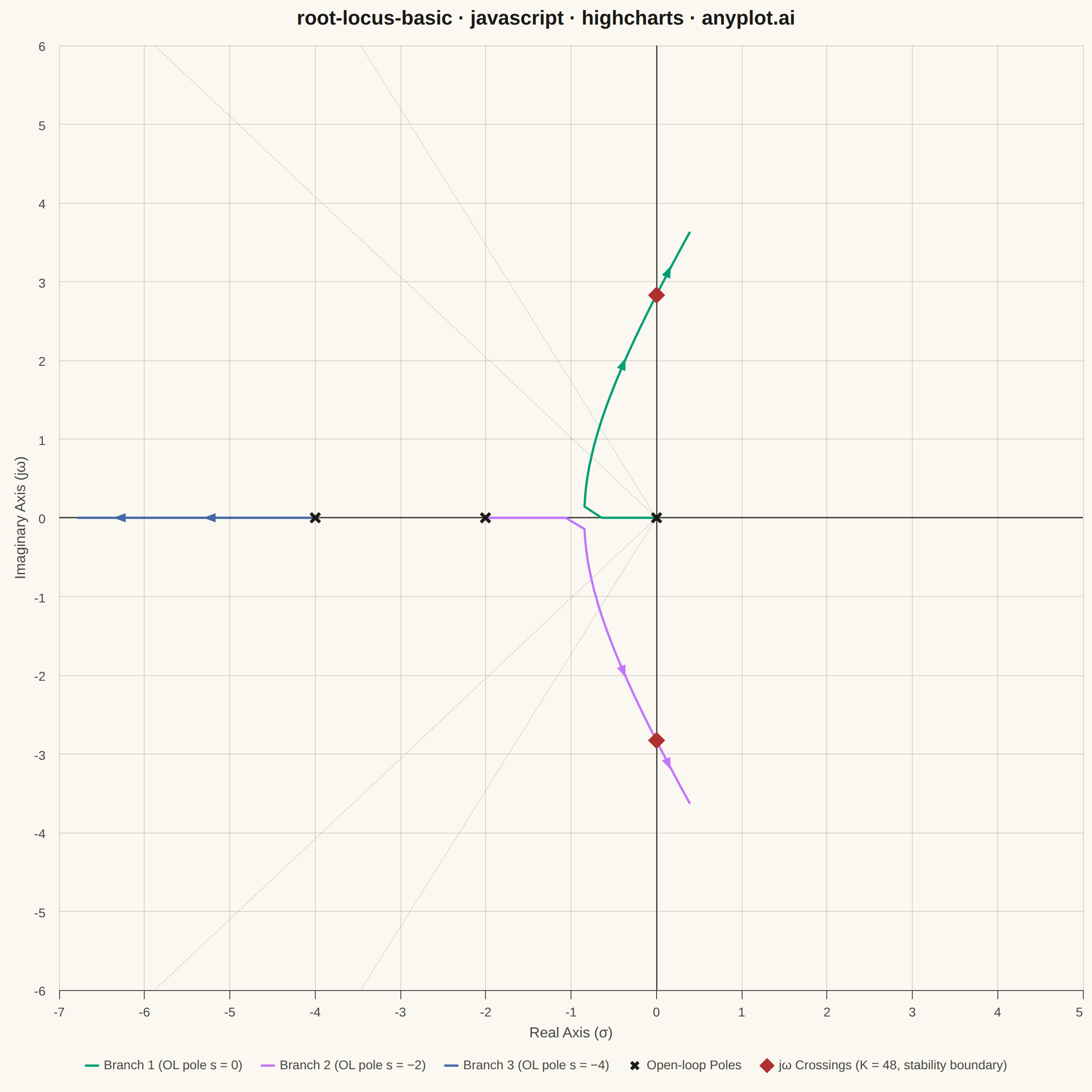
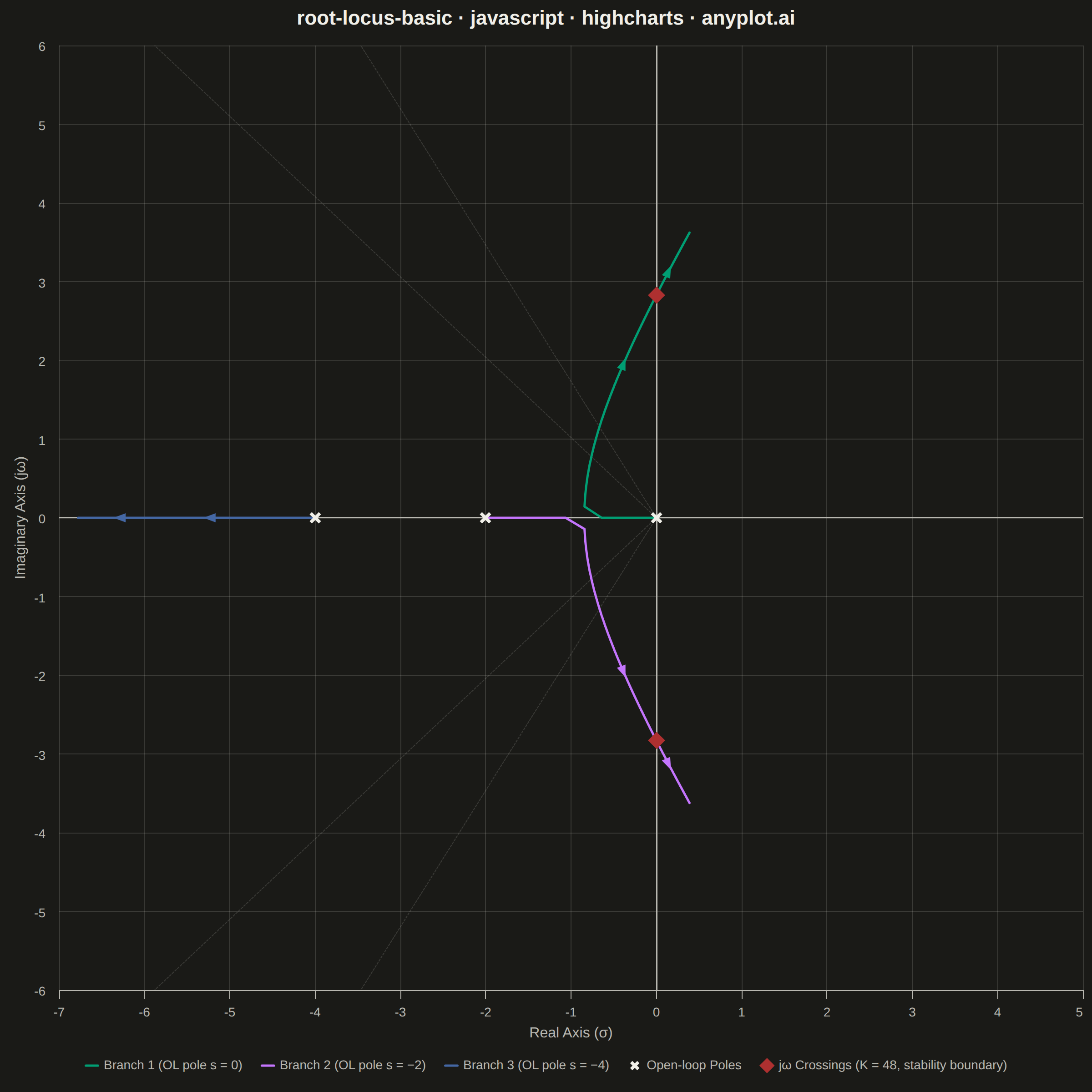
A root locus plot traces how the closed-loop poles of a transfer function migrate through the complex plane as a system parameter (typically gain K) varies from 0 to infinity. It is a fundamental tool in classical control theory for analyzing system stability and designing controllers. The plot reveals critical information about pole trajectories, stability boundaries, and gain margins.
// anyplot.ai
// root-locus-basic: Root Locus Plot for Control Systems
// Library: highcharts 12.6.0 | JavaScript 22.22.3
// Quality: 89/100 | Created: 2026-06-18

//# anyplot-orientation: square

const t = window.ANYPLOT_TOKENS;

// --- Analytic roots for s³ + 6s² + 8s + K = 0 ---------------------------
// Substitution s = t−2 gives depressed cubic t³ − 4t + K = 0.
// disc < 0: three real roots (trigonometric); disc > 0: one real + complex pair (Cardano).
// Returns [[re,im],[re,im],[re,im]] in FIXED branch order across all K:
//   index 0 → pole at  0  (rightmost; upper complex after breakaway)
//   index 1 → pole at −2  (middle;    lower complex after breakaway)
//   index 2 → pole at −4  (leftmost;  always real, goes to −∞)
function cubicRoots(K) {
  const disc = K * K / 4 - 64 / 27;

  if (disc <= 0) {
    // Three real roots via trigonometric method
    const r   = 4 / Math.sqrt(3);
    const arg = Math.max(-1, Math.min(1, -3 * K * Math.sqrt(3) / 16));
    const phi = Math.acos(arg);
    return [
      [r * Math.cos(phi / 3)                - 2, 0],
      [r * Math.cos(phi / 3 - 2 * Math.PI / 3) - 2, 0],
      [r * Math.cos(phi / 3 - 4 * Math.PI / 3) - 2, 0],
    ];
  }

  // One real root + complex conjugate pair (Cardano)
  const D  = Math.sqrt(disc);
  const u1 = -Math.pow(K / 2 - D, 1 / 3); // < 0
  const u2 = -Math.pow(K / 2 + D, 1 / 3); // < 0
  const re = -(u1 + u2) / 2 - 2;           // real part of complex roots
  const im = (Math.sqrt(3) / 2) * (u1 - u2); // imaginary part > 0
  return [
    [re,  im],         // upper complex → branch from pole at  0
    [re, -im],         // lower complex → branch from pole at −2
    [u1 + u2 - 2, 0], // real root     → branch from pole at −4
  ];
}

// --- Root locus data: G(s) = K / (s(s+2)(s+4)) --------------------------
// OL poles: 0, −2, −4  |  No zeros
// Breakaway: s ≈ −0.845, K ≈ 3.08
// Imaginary-axis crossing: K = 48, s = ±j2√2 ≈ ±j2.828
const N_STEPS  = 400;
const K_MAX    = 90;
const branches = [[], [], []];

for (let i = 0; i <= N_STEPS; i++) {
  const K   = (i / N_STEPS) * K_MAX;
  const pts = cubicRoots(K);
  for (let b = 0; b < 3; b++) {
    branches[b].push([+pts[b][0].toFixed(3), +pts[b][1].toFixed(3)]);
  }
}

// --- Custom × marker symbol for open-loop poles --------------------------
Highcharts.SVGRenderer.prototype.symbols.x_pole = function(x, y, w, h) {
  const p = 0.22 * w;
  return [
    'M', x + p,     y + p,     'L', x + w - p, y + h - p,
    'M', x + w - p, y + p,     'L', x + p,     y + h - p,
  ];
};

// --- Series definitions --------------------------------------------------
const branchColors = [t.palette[0], t.palette[1], t.palette[2]]; // canonical palette order
const branchNames  = [
  "Branch 1  (OL pole s = 0)",
  "Branch 2  (OL pole s = −2)",
  "Branch 3  (OL pole s = −4)",
];

const branchSeries = branches.map((pts, b) => ({
  name:      branchNames[b],
  type:      "line",
  data:      pts,
  color:     branchColors[b],
  lineWidth: 2.5,
  marker:    { enabled: false },
  enableMouseTracking: false,
}));

const poleSeries = {
  name:  "Open-loop Poles",
  type:  "scatter",
  data:  [[0, 0], [-2, 0], [-4, 0]],
  color: t.ink,
  marker: {
    symbol:    "x_pole",
    lineWidth: 3.5,
    lineColor: t.ink,
    fillColor: "none",
    radius:    9,
  },
  enableMouseTracking: false,
  zIndex: 5,
};

// Imaginary-axis crossings at K = 48, s = ±j2√2 (stability boundary)
const jOmegaCross = +Math.sqrt(8).toFixed(4);
const crossSeries = {
  name:  "jω Crossings  (K = 48, stability boundary)",
  type:  "scatter",
  data:  [[0, jOmegaCross], [0, -jOmegaCross]],
  color: t.palette[4], // matte red — stability / loss
  marker: { symbol: "diamond", radius: 8, lineWidth: 2, lineColor: t.palette[4] },
  enableMouseTracking: false,
  zIndex: 5,
};

// Constant damping-ratio guide lines (ζ = 0.5, ζ = 0.7), clipped at y = ±6
function dampingLine(zeta, upper) {
  const slope = Math.sqrt(1 - zeta * zeta) / zeta;
  const yLim  = 6;
  const xEnd  = -(yLim / slope);
  return {
    type:      "line",
    data:      [[0, 0], [xEnd, upper ? yLim : -yLim]],
    color:     t.grid,
    lineWidth: 1,
    dashStyle: "ShortDash",
    marker:    { enabled: false },
    enableMouseTracking: false,
    showInLegend: false,
  };
}

const guideSeries = [
  dampingLine(0.5, true),  dampingLine(0.5, false),
  dampingLine(0.7, true),  dampingLine(0.7, false),
];

// --- Chart ---------------------------------------------------------------
const chart = Highcharts.chart("container", {
  chart: {
    backgroundColor: "transparent",
    animation:       false,
    style:           { fontFamily: "inherit" },
  },
  credits: { enabled: false },
  title: {
    text:  "root-locus-basic · javascript · highcharts · anyplot.ai",
    style: { color: t.ink, fontSize: "22px", fontWeight: "600" },
  },
  xAxis: {
    title:         { text: "Real Axis (σ)", style: { color: t.inkSoft, fontSize: "16px" } },
    lineColor:     t.inkSoft,
    tickColor:     t.inkSoft,
    gridLineColor: t.grid,
    gridLineWidth: 1,
    labels:        { style: { color: t.inkSoft, fontSize: "14px" } },
    min: -7, max: 5,
    plotLines: [{ value: 0, color: t.inkSoft, width: 1.5, zIndex: 3 }],
  },
  yAxis: {
    title:         { text: "Imaginary Axis (jω)", style: { color: t.inkSoft, fontSize: "16px" } },
    lineColor:     t.inkSoft,
    tickColor:     t.inkSoft,
    gridLineColor: t.grid,
    gridLineWidth: 1,
    labels:        { style: { color: t.inkSoft, fontSize: "14px" } },
    min: -6, max: 6,
    plotLines: [{ value: 0, color: t.inkSoft, width: 1.5, zIndex: 3 }],
  },
  legend: {
    enabled:        true,
    itemStyle:      { color: t.inkSoft, fontSize: "14px" },
    itemHoverStyle: { color: t.ink },
  },
  plotOptions: { series: { animation: false } },
  series: [...guideSeries, ...branchSeries, poleSeries, crossSeries],
});

// --- Gain-direction arrows (post-render) ---------------------------------
// Filled triangle tips at K=20 and K=60 oriented tangent to each branch,
// indicating the direction of increasing gain as required by the spec.
[20, 60].forEach(arrowK => {
  const idx = Math.round(arrowK / K_MAX * N_STEPS);
  if (idx < 2 || idx >= N_STEPS - 1) return;

  for (let b = 0; b < 3; b++) {
    const [x,  y]  = branches[b][idx];
    const [nx, ny] = branches[b][idx + 1];
    const [px, py] = branches[b][idx - 1];

    const dx = nx - px, dy = ny - py;
    if (dx * dx + dy * dy < 1e-10) return;

    const cx = chart.xAxis[0].toPixels(x, false);
    const cy = chart.yAxis[0].toPixels(y, false);

    // SVG y increases downward, so negate dy for the pixel-space angle
    const θ = Math.atan2(-dy, dx);
    const [cos_θ, sin_θ] = [Math.cos(θ), Math.sin(θ)];
    const [len, w] = [10, 5];

    chart.renderer.path([
      'M', cx + len * cos_θ,                       cy + len * sin_θ,
      'L', cx - (len / 3) * cos_θ - w * sin_θ,     cy - (len / 3) * sin_θ + w * cos_θ,
      'L', cx - (len / 3) * cos_θ + w * sin_θ,     cy - (len / 3) * sin_θ - w * cos_θ,
      'Z',
    ])
      .attr({ fill: branchColors[b], 'stroke-width': 0, zIndex: 6 })
      .add();
  }
});
Runnable source as JSON, for any HTTP client: https://api.anyplot.ai/specs/root-locus-basic/highcharts/code. Any spec id and library id listed in llms-full.txt fit the same URL shape; every URL below is complete and callable.
{
  "spec_id": "root-locus-basic",
  "language": "javascript",
  "library": "highcharts",
  "page": "https://anyplot.ai/root-locus-basic/javascript/highcharts",
  "hub": "https://anyplot.ai/root-locus-basic",
  "code_json": "https://api.anyplot.ai/specs/root-locus-basic/highcharts/code",
  "spec_json": "https://api.anyplot.ai/specs/root-locus-basic",
  "render_light_png": "https://storage.googleapis.com/anyplot-images/plots/root-locus-basic/javascript/highcharts/plot-light.png",
  "render_dark_png": "https://storage.googleapis.com/anyplot-images/plots/root-locus-basic/javascript/highcharts/plot-dark.png",
  "interactive_light_html": "https://storage.googleapis.com/anyplot-images/plots/root-locus-basic/javascript/highcharts/plot-light.html",
  "interactive_dark_html": "https://storage.googleapis.com/anyplot-images/plots/root-locus-basic/javascript/highcharts/plot-dark.html",
  "quality_score": 89.0,
  "license": "MIT",
  "guide": "https://anyplot.ai/llms.txt"
}
Part of Root Locus Plot for Control Systems on anyplot.ai.