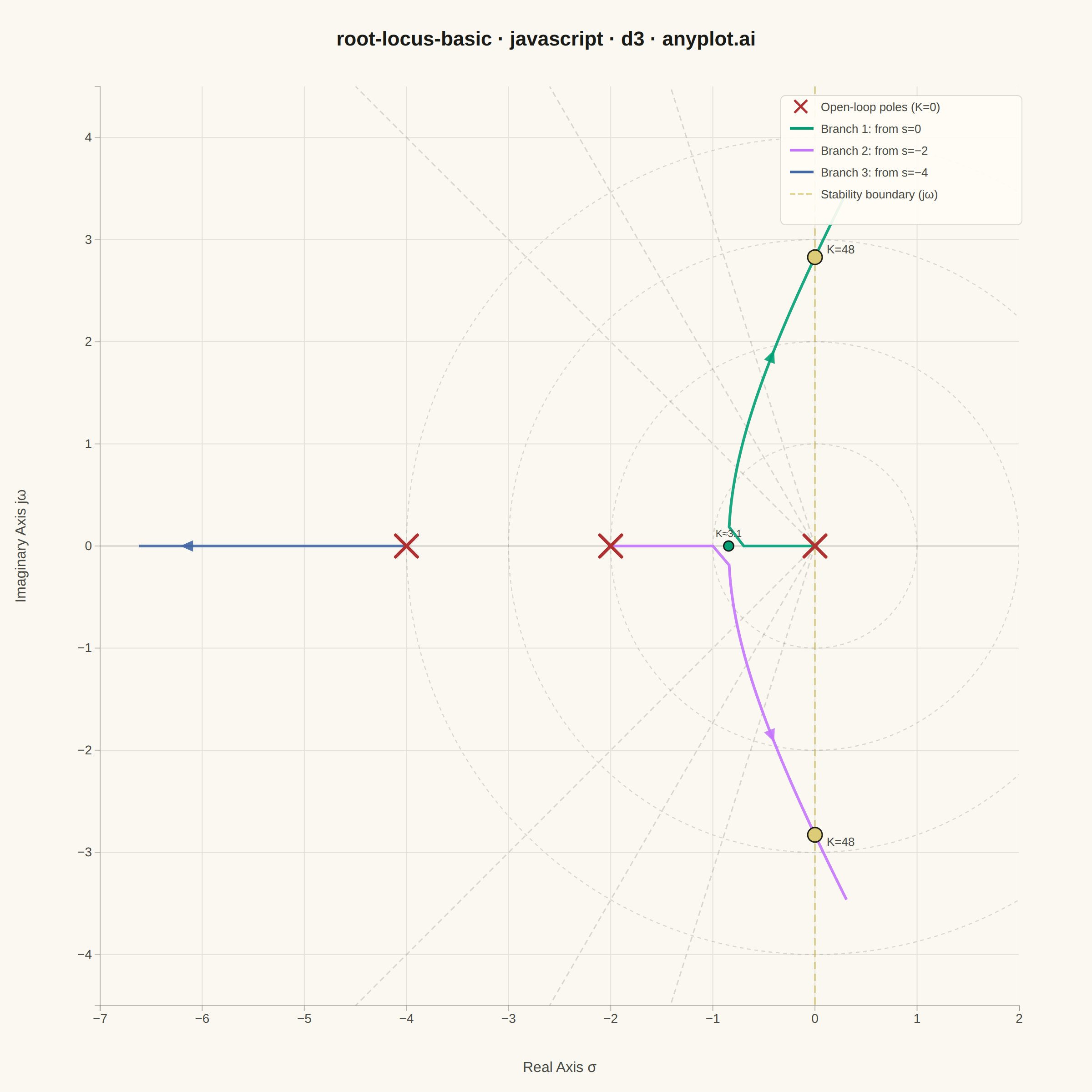
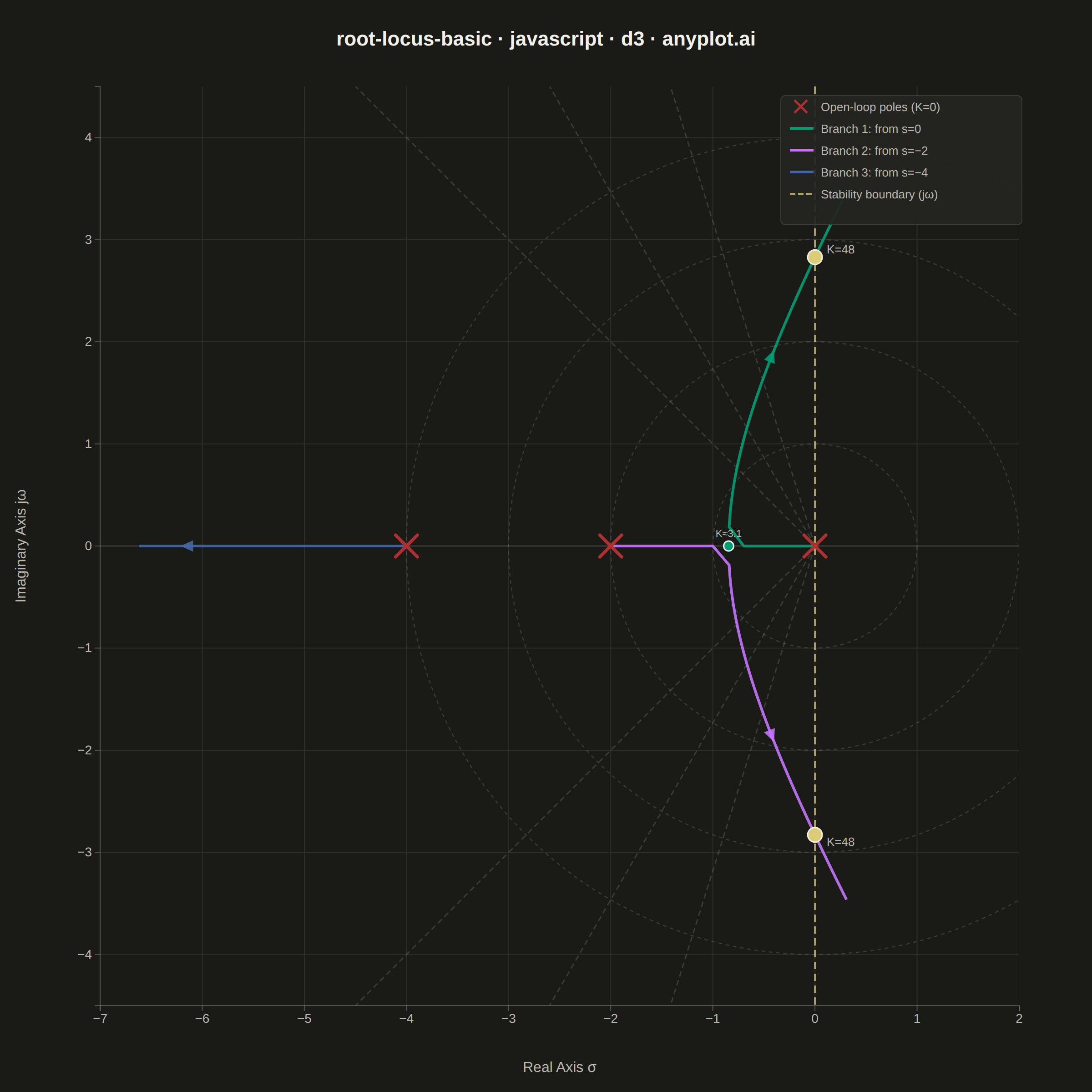
A root locus plot traces how the closed-loop poles of a transfer function migrate through the complex plane as a system parameter (typically gain K) varies from 0 to infinity. It is a fundamental tool in classical control theory for analyzing system stability and designing controllers. The plot reveals critical information about pole trajectories, stability boundaries, and gain margins.
// anyplot.ai
// root-locus-basic: Root Locus Plot for Control Systems
// Library: d3 7.9.0 | JavaScript 22.22.3
// Quality: 88/100 | Created: 2026-06-18

//# anyplot-orientation: square

const t = window.ANYPLOT_TOKENS;
const { width, height } = window.ANYPLOT_SIZE;

// --- Root locus: G(s) = K / [s(s+2)(s+4)] ---------------------------------
// Characteristic equation: s³ + 6s² + 8s + K = 0
// Open-loop poles: 0, −2, −4 | No zeros | 3 branches
// Breakaway: s ≈ −0.845 at K ≈ 3.08 (two real roots merge → complex pair)
// Asymptote centroid: −2 | Angles: 60°, 180°, 300°
// jω-axis crossing: ±j·2√2 ≈ ±j·2.828 at K = 48

// Newton's method: track the monotonically-moving real root (branch 2)
// starting from the root near 'start' as K varies.
function findRealRoot(K, start) {
  let s = start;
  for (let i = 0; i < 200; i++) {
    const ps = s * s * s + 6 * s * s + 8 * s + K;
    const dps = 3 * s * s + 12 * s + 8;
    if (Math.abs(dps) < 1e-15) break;
    const step = ps / dps;
    s -= step;
    if (Math.abs(step) < 1e-12) break;
  }
  return s;
}

// Analytical deflation: divide s³+6s²+8s+K by (s − sReal),
// then solve the resulting quadratic for the other two roots.
// Returns [{upper}, {lower}, {real}] where upper/lower are conjugates past breakaway.
function solveDeflated(sReal) {
  const bq = 6 + sReal;               // quadratic s-coefficient
  const cq = 8 + sReal * (6 + sReal); // quadratic constant
  const disc = bq * bq - 4 * cq;
  if (disc >= 0) {
    const sq = Math.sqrt(disc);
    // Two real roots: larger (branch 0) and smaller (branch 1)
    return [
      { r: (-bq + sq) / 2, i: 0 },
      { r: (-bq - sq) / 2, i: 0 },
      { r: sReal,          i: 0 },
    ];
  }
  // Complex conjugate pair — upper (branch 0) and lower (branch 1)
  const re = -bq / 2;
  const im = Math.sqrt(-disc) / 2;
  return [
    { r: re, i:  im },
    { r: re, i: -im },
    { r: sReal, i: 0 },
  ];
}

const poles = [{ r: 0, i: 0 }, { r: -2, i: 0 }, { r: -4, i: 0 }];
const kSteps = Array.from({ length: 401 }, (_, i) => i * 0.2); // K: 0 → 80
const branches = [[], [], []];
let prevB2 = -4.0; // branch-2 real root starts at pole −4

for (const K of kSteps) {
  const sReal = findRealRoot(K, prevB2);
  prevB2 = sReal;
  const roots = solveDeflated(sReal);
  for (let b = 0; b < 3; b++) branches[b].push({ re: roots[b].r, im: roots[b].i, K });
}

// --- Layout (square canvas: 1200 × 1200 CSS px) ----------------------------
// Equal aspect: iw = ih = 1010, domain = 9 units each → 112 px/unit
const margin = { top: 95, right: 80, bottom: 95, left: 110 };
const iw = width - margin.left - margin.right;
const ih = height - margin.top - margin.bottom;

const svg = d3.select("#container").append("svg").attr("width", width).attr("height", height);
svg.append("defs").append("clipPath").attr("id", "inner")
  .append("rect").attr("width", iw).attr("height", ih);
const g = svg.append("g").attr("transform", `translate(${margin.left},${margin.top})`);

// --- Scales (equal aspect) --------------------------------------------------
const xDom = [-7, 2], yDom = [-4.5, 4.5]; // Both range 9 units
const xs = d3.scaleLinear().domain(xDom).range([0, iw]);
const ys = d3.scaleLinear().domain(yDom).range([ih, 0]);
const unitPx = iw / (xDom[1] - xDom[0]); // ≈ 112 px per unit

// --- Reference: constant ζ lines and ωn circles ----------------------------
const refG = g.append("g").attr("clip-path", "url(#inner)");

const zetaVals = [0.3, 0.5, 0.707];
for (const z of zetaVals) {
  const sinA = Math.sqrt(1 - z * z);
  const tScale = yDom[1] / sinA; // reach top of y-domain
  const ex = Math.max(-z * tScale, xDom[0]);
  const ey = sinA * tScale;
  for (const sign of [1, -1]) {
    refG.append("line")
      .attr("x1", xs(0)).attr("y1", ys(0))
      .attr("x2", xs(ex)).attr("y2", ys(sign * ey))
      .attr("stroke", t.grid).attr("stroke-width", 1.5)
      .attr("stroke-dasharray", "6,4");
  }
  refG.append("text")
    .attr("x", xs(ex) + 4).attr("y", ys(ey) - 4)
    .attr("fill", t.grid).style("font-size", "13px")
    .text(`ζ=${z}`);
}

// Constant ωn circles
for (const wn of [1, 2, 3, 4]) {
  refG.append("circle")
    .attr("cx", xs(0)).attr("cy", ys(0)).attr("r", wn * unitPx)
    .attr("fill", "none").attr("stroke", t.grid)
    .attr("stroke-width", 1.2).attr("stroke-dasharray", "4,4");
}
refG.append("text")
  .attr("x", xs(0) + 2 * unitPx + 4).attr("y", ys(0) + 14)
  .attr("fill", t.grid).style("font-size", "13px").text("ωn=2");
refG.append("text")
  .attr("x", xs(0) + 4 * unitPx + 4).attr("y", ys(0) + 14)
  .attr("fill", t.grid).style("font-size", "13px").text("ωn=4");

// --- Imaginary axis (stability boundary) ------------------------------------
g.append("line")
  .attr("x1", xs(0)).attr("x2", xs(0)).attr("y1", 0).attr("y2", ih)
  .attr("stroke", t.amber).attr("stroke-width", 2)
  .attr("stroke-dasharray", "8,5").attr("opacity", 0.75);

// --- Real axis --------------------------------------------------------------
g.append("line")
  .attr("x1", 0).attr("x2", iw).attr("y1", ys(0)).attr("y2", ys(0))
  .attr("stroke", t.inkSoft).attr("stroke-width", 1).attr("opacity", 0.3);

// --- Integer grid -----------------------------------------------------------
const gridG = g.append("g").attr("clip-path", "url(#inner)").attr("opacity", 0.12);
for (let v = Math.ceil(xDom[0]); v <= Math.floor(xDom[1]); v++) {
  gridG.append("line").attr("x1", xs(v)).attr("x2", xs(v)).attr("y1", 0).attr("y2", ih)
    .attr("stroke", t.inkSoft).attr("stroke-width", 1);
}
for (let v = Math.ceil(yDom[0]); v <= Math.floor(yDom[1]); v++) {
  gridG.append("line").attr("x1", 0).attr("x2", iw).attr("y1", ys(v)).attr("y2", ys(v))
    .attr("stroke", t.inkSoft).attr("stroke-width", 1);
}

// --- Axes -------------------------------------------------------------------
const xAxisG = g.append("g").attr("transform", `translate(0,${ih})`).call(
  d3.axisBottom(xs).ticks(9).tickFormat(d3.format("d"))
);
const yAxisG = g.append("g").call(
  d3.axisLeft(ys).ticks(9).tickFormat(d3.format("d"))
);
for (const ax of [xAxisG, yAxisG]) {
  ax.selectAll("text").attr("fill", t.inkSoft).style("font-size", "14px");
  ax.selectAll("line").attr("stroke", t.inkSoft).attr("opacity", 0.35);
  ax.select(".domain").attr("stroke", t.inkSoft).attr("opacity", 0.35);
}

// --- Root locus branches (clipped) ------------------------------------------
const branchColors = [t.palette[0], t.palette[1], t.palette[2]];
const lineGen = d3.line()
  .x(d => xs(d.re))
  .y(d => ys(d.im))
  .defined(d =>
    isFinite(d.re) && isFinite(d.im)
    && d.re >= xDom[0] - 0.05 && d.re <= xDom[1] + 0.05
    && d.im >= yDom[0] - 0.05 && d.im <= yDom[1] + 0.05
  );

const lociG = g.append("g").attr("clip-path", "url(#inner)");
for (let b = 0; b < 3; b++) {
  lociG.append("path")
    .datum(branches[b])
    .attr("d", lineGen)
    .attr("fill", "none")
    .attr("stroke", branchColors[b])
    .attr("stroke-width", 3)
    .attr("opacity", 0.9);
}

// --- Directional arrows (increasing K) --------------------------------------
function addArrow(grp, cx, cy, dx, dy, color) {
  const len = Math.sqrt(dx * dx + dy * dy);
  if (len < 1) return;
  const ux = dx / len, uy = dy / len, sz = 14;
  const bx = cx - ux * sz, by = cy - uy * sz;
  const nx = -uy * sz * 0.45, ny = ux * sz * 0.45;
  grp.append("polygon")
    .attr("points", `${cx},${cy} ${bx + nx},${by + ny} ${bx - nx},${by - ny}`)
    .attr("fill", color).attr("opacity", 0.9);
}

const arrowG = g.append("g").attr("clip-path", "url(#inner)");
// Arrows at K≈20 for branches 0 & 1 (complex region), K≈58 for branch 2 (real axis)
const arrowK = [20, 20, 58];
for (let b = 0; b < 3; b++) {
  const idx = Math.round(arrowK[b] / 0.2);
  const lo = Math.max(0, idx - 10), hi = Math.min(branches[b].length - 1, idx + 10);
  const pt = branches[b][idx];
  if (!pt) continue;
  addArrow(
    arrowG,
    xs(pt.re), ys(pt.im),
    xs(branches[b][hi].re) - xs(branches[b][lo].re),
    ys(branches[b][hi].im) - ys(branches[b][lo].im),
    branchColors[b]
  );
}

// --- Open-loop pole markers (×) --------------------------------------------
const poleColor = t.palette[4];
const poleG = g.append("g");
for (const p of poles) {
  const px = xs(p.r), py = ys(p.i), s = 12;
  poleG.append("line").attr("x1", px - s).attr("y1", py - s).attr("x2", px + s).attr("y2", py + s)
    .attr("stroke", poleColor).attr("stroke-width", 3.5).attr("stroke-linecap", "round");
  poleG.append("line").attr("x1", px - s).attr("y1", py + s).attr("x2", px + s).attr("y2", py - s)
    .attr("stroke", poleColor).attr("stroke-width", 3.5).attr("stroke-linecap", "round");
}

// --- jω-axis crossing markers (K = 48, s = ±j·2√2) ------------------------
const jwCross = 2 * Math.sqrt(2); // ≈ 2.828
for (const sign of [1, -1]) {
  g.append("circle")
    .attr("cx", xs(0)).attr("cy", ys(sign * jwCross)).attr("r", 8)
    .attr("fill", t.amber).attr("stroke", t.ink).attr("stroke-width", 1.5);
  g.append("text")
    .attr("x", xs(0) + 13).attr("y", ys(sign * jwCross) + (sign > 0 ? -4 : 12))
    .attr("fill", t.inkSoft).style("font-size", "13px")
    .text("K=48");
}

// --- Breakaway point marker -------------------------------------------------
g.append("circle")
  .attr("cx", xs(-0.845)).attr("cy", ys(0)).attr("r", 5.5)
  .attr("fill", t.palette[0]).attr("stroke", t.ink).attr("stroke-width", 1.5);
g.append("text")
  .attr("x", xs(-0.845)).attr("y", ys(0) - 10)
  .attr("text-anchor", "middle").attr("fill", t.inkSoft).style("font-size", "11px")
  .text("K≈3.1");

// --- Legend -----------------------------------------------------------------
const legendItems = [
  { color: poleColor, label: "Open-loop poles (K=0)", type: "x" },
  { color: t.palette[0], label: "Branch 1: from s=0", type: "line" },
  { color: t.palette[1], label: "Branch 2: from s=−2", type: "line" },
  { color: t.palette[2], label: "Branch 3: from s=−4", type: "line" },
  { color: t.amber, label: "Stability boundary (jω)", type: "dash" },
];
const lx = iw - 252, ly0 = 22;
g.append("rect")
  .attr("x", lx - 10).attr("y", ly0 - 12)
  .attr("width", 265).attr("height", legendItems.length * 24 + 22)
  .attr("fill", t.elevatedBg).attr("rx", 5).attr("opacity", 0.92)
  .attr("stroke", t.grid).attr("stroke-width", 1);

legendItems.forEach((item, i) => {
  const liy = ly0 + i * 24;
  if (item.type === "x") {
    const mx = lx + 12, s = 7;
    g.append("line").attr("x1", mx - s).attr("y1", liy - s).attr("x2", mx + s).attr("y2", liy + s)
      .attr("stroke", item.color).attr("stroke-width", 2.5);
    g.append("line").attr("x1", mx - s).attr("y1", liy + s).attr("x2", mx + s).attr("y2", liy - s)
      .attr("stroke", item.color).attr("stroke-width", 2.5);
  } else if (item.type === "dash") {
    g.append("line").attr("x1", lx).attr("y1", liy).attr("x2", lx + 26).attr("y2", liy)
      .attr("stroke", item.color).attr("stroke-width", 2).attr("stroke-dasharray", "6,3").attr("opacity", 0.75);
  } else {
    g.append("line").attr("x1", lx).attr("y1", liy).attr("x2", lx + 26).attr("y2", liy)
      .attr("stroke", item.color).attr("stroke-width", 3);
  }
  g.append("text").attr("x", lx + 34).attr("y", liy + 5)
    .attr("fill", t.inkSoft).style("font-size", "13px").text(item.label);
});

// --- Axis labels ------------------------------------------------------------
svg.append("text")
  .attr("x", margin.left + iw / 2).attr("y", height - 22)
  .attr("text-anchor", "middle").attr("fill", t.inkSoft).style("font-size", "16px")
  .text("Real Axis  σ");

svg.append("text")
  .attr("transform", "rotate(-90)")
  .attr("x", -(margin.top + ih / 2)).attr("y", 28)
  .attr("text-anchor", "middle").attr("fill", t.inkSoft).style("font-size", "16px")
  .text("Imaginary Axis  jω");

// --- Title ------------------------------------------------------------------
svg.append("text")
  .attr("x", width / 2).attr("y", 50)
  .attr("text-anchor", "middle").attr("fill", t.ink)
  .style("font-size", "22px").style("font-weight", "600")
  .text("root-locus-basic · javascript · d3 · anyplot.ai");
Runnable source as JSON, for any HTTP client: https://api.anyplot.ai/specs/root-locus-basic/d3/code. Any spec id and library id listed in llms-full.txt fit the same URL shape; every URL below is complete and callable.
{
  "spec_id": "root-locus-basic",
  "language": "javascript",
  "library": "d3",
  "page": "https://anyplot.ai/root-locus-basic/javascript/d3",
  "hub": "https://anyplot.ai/root-locus-basic",
  "code_json": "https://api.anyplot.ai/specs/root-locus-basic/d3/code",
  "spec_json": "https://api.anyplot.ai/specs/root-locus-basic",
  "render_light_png": "https://storage.googleapis.com/anyplot-images/plots/root-locus-basic/javascript/d3/plot-light.png",
  "render_dark_png": "https://storage.googleapis.com/anyplot-images/plots/root-locus-basic/javascript/d3/plot-dark.png",
  "interactive_light_html": "https://storage.googleapis.com/anyplot-images/plots/root-locus-basic/javascript/d3/plot-light.html",
  "interactive_dark_html": "https://storage.googleapis.com/anyplot-images/plots/root-locus-basic/javascript/d3/plot-dark.html",
  "quality_score": 88.0,
  "license": "MIT",
  "guide": "https://anyplot.ai/llms.txt"
}
Part of Root Locus Plot for Control Systems on anyplot.ai.