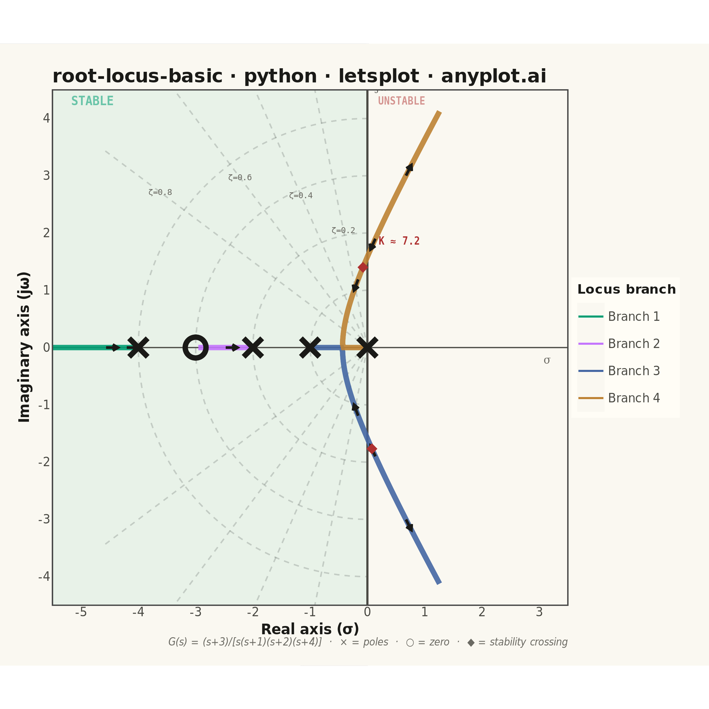
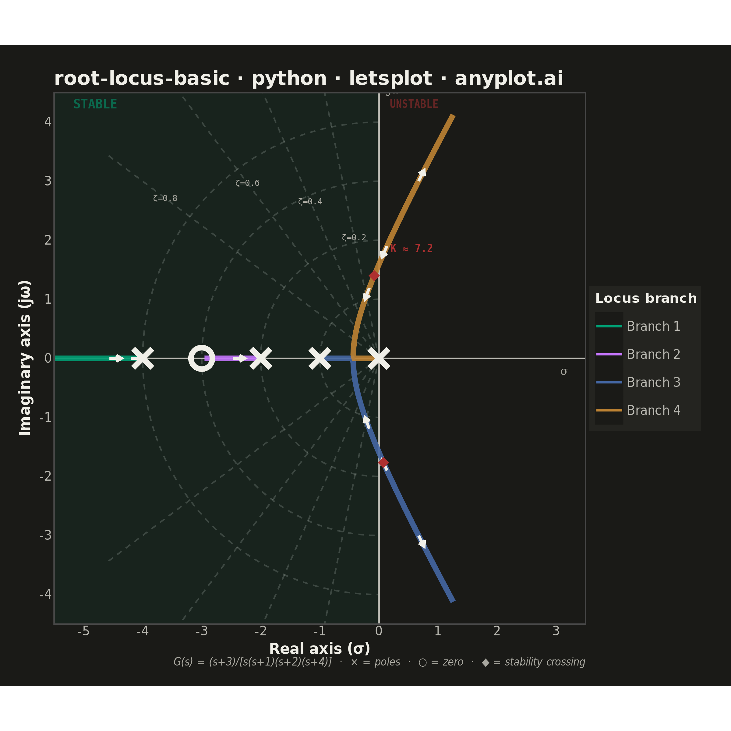
A root locus plot traces how the closed-loop poles of a transfer function migrate through the complex plane as a system parameter (typically gain K) varies from 0 to infinity. It is a fundamental tool in classical control theory for analyzing system stability and designing controllers. The plot reveals critical information about pole trajectories, stability boundaries, and gain margins.
""" anyplot.ai
root-locus-basic: Root Locus Plot for Control Systems
Library: letsplot 4.10.1 | Python 3.13.13
Quality: 86/100 | Updated: 2026-06-18
"""

import os

import numpy as np
import pandas as pd
from lets_plot import *
from lets_plot import aes  # explicit import to satisfy F405 for multi-line calls
from lets_plot.export import ggsave


LetsPlot.setup_html()

# Theme-adaptive chrome — Imprint palette
THEME = os.getenv("ANYPLOT_THEME", "light")
PAGE_BG = "#FAF8F1" if THEME == "light" else "#1A1A17"
ELEVATED_BG = "#FFFDF6" if THEME == "light" else "#242420"
INK = "#1A1A17" if THEME == "light" else "#F0EFE8"
INK_SOFT = "#4A4A44" if THEME == "light" else "#B8B7B0"
INK_MUTED = "#6B6A63" if THEME == "light" else "#A8A79F"
GRID_RULE = "rgba(26,26,23,0.18)" if THEME == "light" else "rgba(240,239,232,0.18)"

# Imprint categorical palette — hybrid-v3 canonical order
IMPRINT_PALETTE = ["#009E73", "#C475FD", "#4467A3", "#BD8233", "#AE3030", "#2ABCCD", "#954477", "#99B314"]

# Data — G(s) = (s + 3) / [s(s+1)(s+2)(s+4)]
# Open-loop poles: 0, −1, −2, −4 | Open-loop zero: −3
den_coeffs = np.polymul(np.polymul([1, 0], [1, 1]), np.polymul([1, 2], [1, 4]))

open_loop_poles = np.array([0.0, -1.0, -2.0, -4.0])
open_loop_zeros = np.array([-3.0])

# Gain sweep: dense near origin to capture breakaway, sparser at high gain
k_values = np.concatenate(
    [np.linspace(0, 0.5, 200), np.linspace(0.5, 5, 400), np.linspace(5, 30, 400), np.linspace(30, 120, 400)]
)

all_real, all_imag, all_gain, all_branch = [], [], [], []
for k in k_values:
    char_poly = np.polyadd(den_coeffs, k * np.array([0, 0, 0, 1, 3]))
    roots = np.sort_complex(np.roots(char_poly))
    for b, root in enumerate(roots):
        all_real.append(root.real)
        all_imag.append(root.imag)
        all_gain.append(k)
        all_branch.append(f"Branch {b + 1}")

df = pd.DataFrame({"real": all_real, "imaginary": all_imag, "gain": all_gain, "branch": all_branch})

# Pole and zero marker data
poles_df = pd.DataFrame({"real": open_loop_poles, "imaginary": 0.0})
zeros_df = pd.DataFrame({"real": open_loop_zeros, "imaginary": 0.0})

# Imaginary-axis stability crossings (real ≈ 0, nonzero imaginary part)
crossing_mask = (np.abs(df["real"]) < 0.08) & (np.abs(df["imaginary"]) > 0.3)
crossings = df[crossing_mask].copy()
if len(crossings) > 0:
    crossings = crossings.sort_values("imaginary")
    crossing_pts = pd.concat(
        [crossings[crossings["imaginary"] > 0].head(1), crossings[crossings["imaginary"] < 0].head(1)]
    )
else:
    crossing_pts = pd.DataFrame(columns=df.columns)

# Direction arrows at selected gain values
arrow_gains = [5, 15, 50]
arrow_rows = []
for ag in arrow_gains:
    idx = np.argmin(np.abs(k_values - ag))
    subset = df[(df["gain"] >= k_values[max(0, idx - 1)]) & (df["gain"] <= k_values[min(len(k_values) - 1, idx + 1)])]
    for _, row in subset.drop_duplicates(subset="branch").iterrows():
        k_next = k_values[min(len(k_values) - 1, idx + 5)]
        next_pts = df[(np.abs(df["gain"] - k_next) < 1.0) & (df["branch"] == row["branch"])]
        if len(next_pts) > 0:
            npt = next_pts.iloc[0]
            dx, dy = npt["real"] - row["real"], npt["imaginary"] - row["imaginary"]
            mag = np.hypot(dx, dy)
            if mag > 0.01:
                s = 0.25 / mag
                arrow_rows.append(
                    {
                        "x": row["real"],
                        "y": row["imaginary"],
                        "xend": row["real"] + dx * s,
                        "yend": row["imaginary"] + dy * s,
                    }
                )
arrows_df = pd.DataFrame(arrow_rows) if arrow_rows else pd.DataFrame(columns=["x", "y", "xend", "yend"])

# Damping ratio guide lines (ζ = constant), radial from origin in LHP
r_max = 5.8
zeta_values = [0.2, 0.4, 0.6, 0.8]
zeta_segs = []
for z in zeta_values:
    theta = np.arccos(z)
    zeta_segs += [
        {"x": 0, "y": 0, "xend": -r_max * np.cos(theta), "yend": r_max * np.sin(theta)},
        {"x": 0, "y": 0, "xend": -r_max * np.cos(theta), "yend": -r_max * np.sin(theta)},
    ]
zeta_df = pd.DataFrame(zeta_segs)

# Zeta labels — staggered radial distances to avoid crowding in upper LHP
zeta_labels = pd.DataFrame(
    [
        {
            "x": -r_max * (0.36 + i * 0.14) * np.cos(np.arccos(z)),
            "y": r_max * (0.36 + i * 0.14) * np.sin(np.arccos(z)),
            "label": f"ζ={z}",
        }
        for i, z in enumerate(zeta_values)
    ]
)

# Natural frequency arcs (ωn = constant semicircles, LHP only)
wn_values = [1, 2, 3, 4]
wn_rows = []
for wn in wn_values:
    theta = np.linspace(np.pi / 2, 3 * np.pi / 2, 120)
    wn_rows += [{"real": wn * np.cos(t), "imaginary": wn * np.sin(t), "wn": str(wn)} for t in theta]
wn_df = pd.DataFrame(wn_rows)

# Critical gain annotation at stability boundary
crit_k = crossing_pts["gain"].iloc[0] if len(crossing_pts) > 0 else None
crit_y = float(crossing_pts["imaginary"].max()) if len(crossing_pts) > 0 else 2.0
annot_df = pd.DataFrame(
    {"x": [0.2], "y": [crit_y + 0.45], "label": [f"K ≈ {crit_k:.1f}" if crit_k is not None else ""]}
)

plot = (
    ggplot()
    # ── Reference overlays (behind data) ───────────────────────────────
    + geom_path(
        aes(x="real", y="imaginary", group="wn"),
        data=wn_df,
        color=GRID_RULE,
        size=0.5,
        linetype="dashed",
        tooltips="none",
    )
    + geom_segment(
        aes(x="x", y="y", xend="xend", yend="yend"),
        data=zeta_df,
        color=GRID_RULE,
        size=0.5,
        linetype="dashed",
        tooltips="none",
    )
    # Stable LHP shading with Imprint brand green tint
    + geom_rect(
        aes(xmin="xmin", ymin="ymin", xmax="xmax", ymax="ymax"),
        data=pd.DataFrame({"xmin": [-6.5], "xmax": [0.0], "ymin": [-5.5], "ymax": [5.5]}),
        fill=IMPRINT_PALETTE[0],
        alpha=0.07,
        inherit_aes=False,
        tooltips="none",
    )
    # ── Axis reference lines ────────────────────────────────────────────
    + geom_vline(xintercept=0, color=INK_SOFT, size=0.7)
    + geom_hline(yintercept=0, color=INK_SOFT, size=0.4)
    # ── Locus branches (Imprint palette, interactive tooltips) ──────────
    + geom_path(
        aes(x="real", y="imaginary", color="branch"),
        data=df,
        size=2.0,
        alpha=0.9,
        tooltips=layer_tooltips()
        .format("gain", ".2f")
        .format("real", ".3f")
        .format("imaginary", ".3f")
        .line("Branch @branch")
        .line("K = @gain")
        .line("Re = @real")
        .line("Im = @imaginary"),
    )
    + scale_color_manual(values=IMPRINT_PALETTE[:4], name="Locus branch")
    # ── Direction arrows (increasing gain) ─────────────────────────────
    + geom_segment(
        aes(x="x", y="y", xend="xend", yend="yend"),
        data=arrows_df,
        color=INK,
        size=1.0,
        inherit_aes=False,
        tooltips="none",
        arrow=arrow(length=10, ends="last", type="open"),
    )
    # ── Open-loop poles (×) and zero (○) ───────────────────────────────
    + geom_point(
        aes(x="real", y="imaginary"),
        data=poles_df,
        shape=4,
        size=6,
        color=INK,
        stroke=2.0,
        inherit_aes=False,
        tooltips=layer_tooltips().line("Pole: s = @real"),
    )
    + geom_point(
        aes(x="real", y="imaginary"),
        data=zeros_df,
        shape=1,
        size=6,
        color=INK,
        stroke=2.0,
        inherit_aes=False,
        tooltips=layer_tooltips().line("Zero: s = @real"),
    )
    # ── Stability-boundary crossings ────────────────────────────────────
    + geom_point(
        aes(x="real", y="imaginary"),
        data=crossing_pts,
        shape=18,
        size=6,
        color=IMPRINT_PALETTE[4],
        inherit_aes=False,
        tooltips=layer_tooltips().line("Stability boundary").line("K ≈ @gain"),
    )
    # ── Text annotations ────────────────────────────────────────────────
    # Zeta labels — staggered for legibility
    + geom_text(
        aes(x="x", y="y", label="label"),
        data=zeta_labels,
        size=3.5,
        color=INK_MUTED,
        inherit_aes=False,
        family="monospace",
    )
    # Complex-plane axis symbols
    + geom_text(
        aes(x="x", y="y", label="label"),
        data=pd.DataFrame({"x": [0.15], "y": [4.55], "label": ["jω"]}),
        size=4.5,
        color=INK_MUTED,
        hjust=0,
        family="serif",
        inherit_aes=False,
    )
    + geom_text(
        aes(x="x", y="y", label="label"),
        data=pd.DataFrame({"x": [3.2], "y": [-0.22], "label": ["σ"]}),
        size=4.5,
        color=INK_MUTED,
        hjust=1,
        family="serif",
        inherit_aes=False,
    )
    # Stability region labels
    + geom_text(
        aes(x="x", y="y", label="label"),
        data=pd.DataFrame({"x": [-4.8], "y": [4.3], "label": ["STABLE"]}),
        size=5.0,
        color=IMPRINT_PALETTE[0],
        alpha=0.55,
        fontface="bold",
        family="monospace",
        inherit_aes=False,
    )
    + geom_text(
        aes(x="x", y="y", label="label"),
        data=pd.DataFrame({"x": [0.6], "y": [4.3], "label": ["UNSTABLE"]}),
        size=4.0,
        color=IMPRINT_PALETTE[4],
        alpha=0.5,
        fontface="bold",
        family="monospace",
        inherit_aes=False,
    )
    # Critical gain annotation
    + geom_text(
        aes(x="x", y="y", label="label"),
        data=annot_df,
        size=4.0,
        color=IMPRINT_PALETTE[4],
        hjust=0,
        family="monospace",
        fontface="bold",
        inherit_aes=False,
    )
    # ── Title, axis labels, layout ──────────────────────────────────────
    + labs(
        x="Real axis (σ)",
        y="Imaginary axis (jω)",
        title="root-locus-basic · python · letsplot · anyplot.ai",
        caption="G(s) = (s+3)/[s(s+1)(s+2)(s+4)]  ·  × = poles  ·  ○ = zero  ·  ◆ = stability crossing",
    )
    # Equal-axis scaling preserves geometry (circles stay circular)
    + coord_fixed(ratio=1, xlim=[-5.5, 3.5], ylim=[-4.5, 4.5])
    + ggsize(600, 600)
    + theme_minimal()
    + theme(
        axis_text=element_text(size=10, color=INK_SOFT),
        axis_title=element_text(size=12, color=INK, face="bold"),
        plot_title=element_text(size=16, color=INK, face="bold"),
        plot_caption=element_text(size=9, color=INK_MUTED, face="italic"),
        legend_text=element_text(size=10, color=INK_SOFT),
        legend_title=element_text(size=11, color=INK, face="bold"),
        legend_position="right",
        panel_grid_major=element_blank(),
        panel_grid_minor=element_blank(),
        plot_background=element_rect(fill=PAGE_BG, color=PAGE_BG),
        panel_background=element_rect(fill=PAGE_BG),
        axis_line=element_line(color=INK_SOFT, size=0.5),
        legend_background=element_rect(fill=ELEVATED_BG, color=INK_SOFT),
        plot_margin=[20, 25, 15, 15],
    )
)

# Save PNG (scale=4 → 2400 × 2400) and interactive HTML
ggsave(plot, f"plot-{THEME}.png", path=".", scale=4)
ggsave(plot, f"plot-{THEME}.html", path=".")
Runnable source as JSON, for any HTTP client: https://api.anyplot.ai/specs/root-locus-basic/letsplot/code. Any spec id and library id listed in llms-full.txt fit the same URL shape; every URL below is complete and callable.
{
  "spec_id": "root-locus-basic",
  "language": "python",
  "library": "letsplot",
  "page": "https://anyplot.ai/root-locus-basic/python/letsplot",
  "hub": "https://anyplot.ai/root-locus-basic",
  "code_json": "https://api.anyplot.ai/specs/root-locus-basic/letsplot/code",
  "spec_json": "https://api.anyplot.ai/specs/root-locus-basic",
  "render_light_png": "https://storage.googleapis.com/anyplot-images/plots/root-locus-basic/python/letsplot/plot-light.png",
  "render_dark_png": "https://storage.googleapis.com/anyplot-images/plots/root-locus-basic/python/letsplot/plot-dark.png",
  "interactive_light_html": "https://storage.googleapis.com/anyplot-images/plots/root-locus-basic/python/letsplot/plot-light.html",
  "interactive_dark_html": "https://storage.googleapis.com/anyplot-images/plots/root-locus-basic/python/letsplot/plot-dark.html",
  "quality_score": 86.0,
  "license": "MIT",
  "guide": "https://anyplot.ai/llms.txt"
}
Part of Root Locus Plot for Control Systems on anyplot.ai.