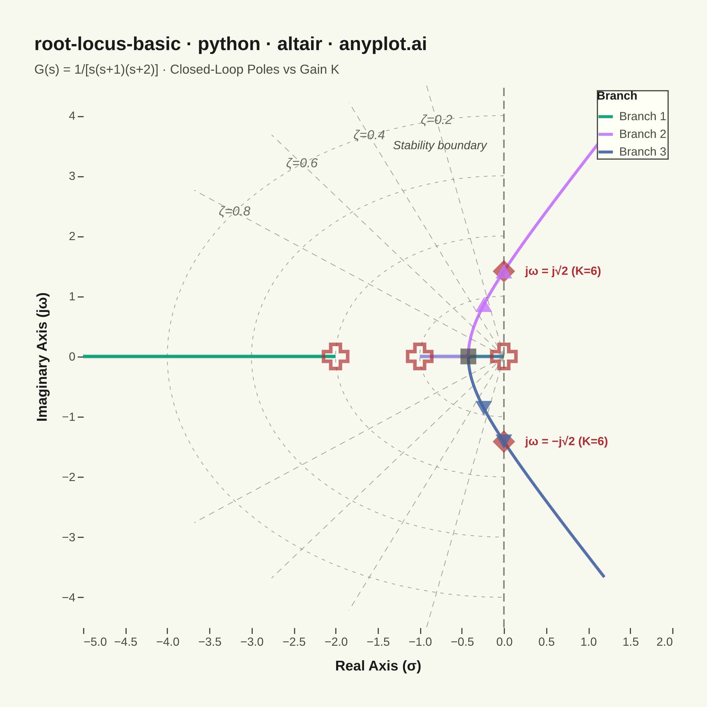
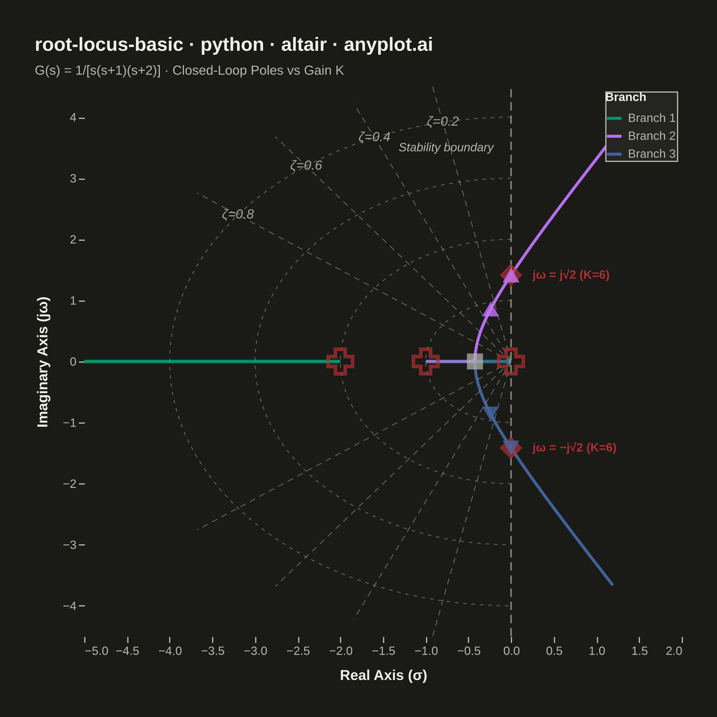
A root locus plot traces how the closed-loop poles of a transfer function migrate through the complex plane as a system parameter (typically gain K) varies from 0 to infinity. It is a fundamental tool in classical control theory for analyzing system stability and designing controllers. The plot reveals critical information about pole trajectories, stability boundaries, and gain margins.
""" anyplot.ai
root-locus-basic: Root Locus Plot for Control Systems
Library: altair 6.2.1 | Python 3.13.13
Quality: 88/100 | Updated: 2026-06-18
"""

import os
import sys


# Prevent this file from shadowing the installed altair package when Python
# prepends the script's directory to sys.path (standard `python altair.py` behavior).
_impl_dir = os.path.dirname(os.path.abspath(__file__))
sys.path = [p for p in sys.path if os.path.abspath(p if p else ".") != _impl_dir]

import altair as alt
import numpy as np
import pandas as pd
from PIL import Image


# Theme tokens
THEME = os.getenv("ANYPLOT_THEME", "light")
PAGE_BG = "#FAF8F1" if THEME == "light" else "#1A1A17"
ELEVATED_BG = "#FFFDF6" if THEME == "light" else "#242420"
INK = "#1A1A17" if THEME == "light" else "#F0EFE8"
INK_SOFT = "#4A4A44" if THEME == "light" else "#B8B7B0"
INK_MUTED = "#6B6A63" if THEME == "light" else "#A8A79F"

# Imprint palette — branch colors (positions 1→3)
IMPRINT_PALETTE = ["#009E73", "#C475FD", "#4467A3", "#BD8233", "#AE3030", "#2ABCCD", "#954477", "#99B314"]
POLE_COLOR = "#AE3030"  # semantic anchor: marks critical/boundary locations

# Data — G(s) = 1 / [s(s+1)(s+2)], open-loop poles at 0, −1, −2
den_coeffs = [1.0, 3.0, 2.0, 0.0]

gains = np.concatenate(
    [
        np.linspace(0.001, 0.5, 150),
        np.linspace(0.5, 2, 200),
        np.linspace(2, 6, 150),
        np.linspace(6, 20, 150),
        np.linspace(20, 80, 100),
    ]
)
n_roots = 3
all_roots = np.zeros((len(gains), n_roots), dtype=complex)

for i, k in enumerate(gains):
    poly = np.array(den_coeffs, dtype=float)
    poly[-1] += k
    all_roots[i] = np.roots(poly)

# Sort into continuous branches via nearest-neighbor matching
all_roots[0] = np.sort(all_roots[0].real)
for i in range(1, len(gains)):
    prev, curr = all_roots[i - 1], all_roots[i]
    dist = np.abs(prev[:, None] - curr[None, :])
    order = np.zeros(n_roots, dtype=int)
    used = set()
    for j in range(n_roots):
        dists = [(dist[j, m], m) for m in range(n_roots) if m not in used]
        _, best = min(dists)
        used.add(best)
        order[j] = best
    all_roots[i] = curr[order]

# Build branch dataframe
rows = []
for b in range(n_roots):
    for i in range(len(gains)):
        rows.append(
            {
                "real": float(all_roots[i, b].real),
                "imaginary": float(all_roots[i, b].imag),
                "gain": float(gains[i]),
                "branch": f"Branch {b + 1}",
                "idx": i,
            }
        )
locus_df = pd.DataFrame(rows)

# Open-loop poles (× markers)
poles_df = pd.DataFrame(
    {"real": [0.0, -1.0, -2.0], "imaginary": [0.0, 0.0, 0.0], "label": ["Pole (s=0)", "Pole (s=−1)", "Pole (s=−2)"]}
)

# Imaginary axis crossing: ω = √2, K = 6
omega_cross = np.sqrt(2)
crossing_df = pd.DataFrame(
    {"real": [0.0, 0.0], "imaginary": [omega_cross, -omega_cross], "label": ["jω = j√2 (K=6)", "jω = −j√2 (K=6)"]}
)

# Breakaway point: 3s²+6s+2 = 0 → s ≈ −0.423
breakaway_df = pd.DataFrame({"bx": [(-6 + np.sqrt(12)) / 6], "by": [0.0], "label": ["Breakaway (s ≈ −0.42)"]})

# Damping ratio guide lines — all four values, both half-planes
damping_rows = []
for zeta in [0.2, 0.4, 0.6, 0.8]:
    angle = np.pi - np.arccos(zeta)
    for side, sign in [("upper", 1), ("lower", -1)]:
        seg = f"zeta_{zeta}_{side}"
        damping_rows.append({"gx": 0.0, "gy": 0.0, "seg": seg, "ord": 0})
        damping_rows.append({"gx": 4.6 * np.cos(angle), "gy": sign * 4.6 * np.sin(angle), "seg": seg, "ord": 1})
damping_df = pd.DataFrame(damping_rows)

# Damping labels — all 4 values on upper side
damping_label_rows = []
for zeta in [0.2, 0.4, 0.6, 0.8]:
    angle = np.pi - np.arccos(zeta)
    damping_label_rows.append({"lx": 4.0 * np.cos(angle), "ly": 4.0 * np.sin(angle), "label": f"ζ={zeta}"})
damping_label_df = pd.DataFrame(damping_label_rows)

# Natural frequency arcs (ωn = 1, 2, 3, 4) — left half-plane semicircles
wn_rows = []
for wn in [1.0, 2.0, 3.0, 4.0]:
    theta = np.linspace(np.pi / 2, 3 * np.pi / 2, 60)
    for j, t in enumerate(theta):
        wn_rows.append({"gx": wn * np.cos(t), "gy": wn * np.sin(t), "wn": f"ωn={wn}", "ord": j})
wn_df = pd.DataFrame(wn_rows)

# Real axis segments: (−1, 0) and (−∞, −2)
real_axis_df = pd.DataFrame(
    {
        "rx": [-1.0, 0.0, -5.0, -2.0],
        "ry": [0.0, 0.0, 0.0, 0.0],
        "seg": ["seg1", "seg1", "seg2", "seg2"],
        "ord": [0, 1, 0, 1],
    }
)

# Gain-direction arrows on complex branches
arrows = []
for b in range(n_roots):
    for idx in [350, 500]:
        if idx + 5 < len(gains):
            r0 = all_roots[idx, b]
            if abs(r0.imag) > 0.3:
                arrows.append({"ax": float(r0.real), "ay": float(r0.imag), "branch": f"Branch {b + 1}"})
arrow_df = pd.DataFrame(arrows) if arrows else pd.DataFrame({"ax": [], "ay": [], "branch": []})

# Stability boundary at imaginary axis (x=0) — key insight for non-control-theory readers
stability_line_df = pd.DataFrame({"sx": [0.0, 0.0], "sy": [-4.5, 4.5], "ord": [0, 1]})
stability_label_df = pd.DataFrame({"sx": [-0.12], "sy": [3.5], "label": ["Stability boundary"]})

# Scales — shift x domain left to reduce empty right-half-plane space
x_scale = alt.Scale(domain=[-5.0, 2.0], nice=False)
y_scale = alt.Scale(domain=[-4.5, 4.5], nice=False)

branch_domain = ["Branch 1", "Branch 2", "Branch 3"]
branch_palette = IMPRINT_PALETTE[:3]

# Title — length 48, under 67 baseline, no scaling needed
title_str = "root-locus-basic · python · altair · anyplot.ai"

# Axis config for locus layer (font sizes; colors via configure_axis)
ax_cfg = {"labelFontSize": 10, "titleFontSize": 12, "grid": False, "titlePadding": 10}

# Layers
locus_layer = (
    alt.Chart(locus_df)
    .mark_line(strokeWidth=2.5, opacity=0.92)
    .encode(
        x=alt.X("real:Q", scale=x_scale, title="Real Axis (σ)", axis=alt.Axis(**ax_cfg)),
        y=alt.Y("imaginary:Q", scale=y_scale, title="Imaginary Axis (jω)", axis=alt.Axis(**ax_cfg)),
        color=alt.Color(
            "branch:N",
            scale=alt.Scale(domain=branch_domain, range=branch_palette),
            legend=alt.Legend(
                title="Branch",
                titleFontSize=10,
                labelFontSize=10,
                symbolSize=150,
                symbolStrokeWidth=2.5,
                orient="top-right",
                offset=4,
            ),
        ),
        order="idx:Q",
        tooltip=[
            alt.Tooltip("branch:N", title="Branch"),
            alt.Tooltip("real:Q", title="σ", format=".3f"),
            alt.Tooltip("imaginary:Q", title="jω", format=".3f"),
            alt.Tooltip("gain:Q", title="Gain K", format=".2f"),
        ],
    )
)

damping_layer = (
    alt.Chart(damping_df)
    .mark_line(strokeWidth=0.7, strokeDash=[5, 4], color=INK_MUTED, opacity=0.55)
    .encode(x=alt.X("gx:Q", scale=x_scale), y=alt.Y("gy:Q", scale=y_scale), detail="seg:N", order="ord:Q")
)

damping_label_layer = (
    alt.Chart(damping_label_df)
    .mark_text(fontSize=11, color=INK_MUTED, fontStyle="italic", align="center")
    .encode(x=alt.X("lx:Q", scale=x_scale), y=alt.Y("ly:Q", scale=y_scale), text="label:N")
)

wn_layer = (
    alt.Chart(wn_df)
    .mark_line(strokeWidth=0.7, strokeDash=[3, 4], color=INK_MUTED, opacity=0.55)
    .encode(x=alt.X("gx:Q", scale=x_scale), y=alt.Y("gy:Q", scale=y_scale), detail="wn:N", order="ord:Q")
)

real_axis_layer = (
    alt.Chart(real_axis_df)
    .mark_line(strokeWidth=4, color=IMPRINT_PALETTE[0], opacity=0.2)
    .encode(x=alt.X("rx:Q", scale=x_scale), y=alt.Y("ry:Q", scale=y_scale), detail="seg:N", order="ord:Q")
)

stability_line_layer = (
    alt.Chart(stability_line_df)
    .mark_line(strokeWidth=1.3, strokeDash=[7, 4], color=INK_SOFT, opacity=0.65)
    .encode(x=alt.X("sx:Q", scale=x_scale), y=alt.Y("sy:Q", scale=y_scale), order="ord:Q")
)

stability_label_layer = (
    alt.Chart(stability_label_df)
    .mark_text(fontSize=10, color=INK_SOFT, align="right", fontStyle="italic", dx=-6)
    .encode(x=alt.X("sx:Q", scale=x_scale), y=alt.Y("sy:Q", scale=y_scale), text="label:N")
)

poles_layer = (
    alt.Chart(poles_df)
    .mark_point(shape="cross", size=420, strokeWidth=3, color=POLE_COLOR, filled=False)
    .encode(
        x=alt.X("real:Q", scale=x_scale),
        y=alt.Y("imaginary:Q", scale=y_scale),
        tooltip=[alt.Tooltip("label:N", title="")],
    )
)

crossing_layer = (
    alt.Chart(crossing_df)
    .mark_point(shape="diamond", size=360, strokeWidth=2, color=POLE_COLOR, filled=True)
    .encode(
        x=alt.X("real:Q", scale=x_scale),
        y=alt.Y("imaginary:Q", scale=y_scale),
        tooltip=[alt.Tooltip("label:N", title="Crossing")],
    )
)

crossing_text = (
    alt.Chart(crossing_df)
    .mark_text(fontSize=10, fontWeight="bold", color=POLE_COLOR, align="left", dx=18)
    .encode(x=alt.X("real:Q", scale=x_scale), y=alt.Y("imaginary:Q", scale=y_scale), text="label:N")
)

breakaway_layer = (
    alt.Chart(breakaway_df)
    .mark_point(shape="square", size=180, color=INK_SOFT, filled=True, opacity=0.7)
    .encode(
        x=alt.X("bx:Q", scale=x_scale), y=alt.Y("by:Q", scale=y_scale), tooltip=[alt.Tooltip("label:N", title="Point")]
    )
)

arrow_up_df = arrow_df[arrow_df["ay"] > 0] if len(arrow_df) > 0 else arrow_df
arrow_down_df = arrow_df[arrow_df["ay"] <= 0] if len(arrow_df) > 0 else arrow_df

arrow_up_layer = (
    alt.Chart(arrow_up_df)
    .mark_point(shape="triangle-up", size=200, filled=True, opacity=0.8)
    .encode(
        x=alt.X("ax:Q", scale=x_scale),
        y=alt.Y("ay:Q", scale=y_scale),
        color=alt.Color("branch:N", scale=alt.Scale(domain=branch_domain, range=branch_palette), legend=None),
    )
)

arrow_down_layer = (
    alt.Chart(arrow_down_df)
    .mark_point(shape="triangle-down", size=200, filled=True, opacity=0.8)
    .encode(
        x=alt.X("ax:Q", scale=x_scale),
        y=alt.Y("ay:Q", scale=y_scale),
        color=alt.Color("branch:N", scale=alt.Scale(domain=branch_domain, range=branch_palette), legend=None),
    )
)

# Compose all layers
chart = (
    (
        stability_line_layer
        + stability_label_layer
        + locus_layer
        + damping_layer
        + damping_label_layer
        + wn_layer
        + real_axis_layer
        + poles_layer
        + crossing_layer
        + crossing_text
        + breakaway_layer
        + arrow_up_layer
        + arrow_down_layer
    )
    .properties(
        width=500,
        height=460,
        background=PAGE_BG,
        title=alt.Title(
            title_str,
            fontSize=16,
            fontWeight="bold",
            color=INK,
            subtitle="G(s) = 1/[s(s+1)(s+2)]  ·  Closed-Loop Poles vs Gain K",
            subtitleFontSize=11,
            subtitleColor=INK_SOFT,
            subtitlePadding=8,
            anchor="start",
            offset=8,
        ),
    )
    .configure_view(fill=PAGE_BG, stroke=None, strokeWidth=0)
    .configure_axis(domain=False, tickColor=INK_SOFT, labelColor=INK_SOFT, titleColor=INK)
    .configure_title(color=INK)
    .configure_legend(fillColor=ELEVATED_BG, strokeColor=INK_SOFT, labelColor=INK_SOFT, titleColor=INK)
    .interactive()
)

# Save PNG
chart.save(f"plot-{THEME}.png", scale_factor=4.0)

# Pad to exact 2400×2400 (square target for root locus)
TW, TH = 2400, 2400
_img = Image.open(f"plot-{THEME}.png").convert("RGB")
_w, _h = _img.size
if _w > TW or _h > TH:
    raise SystemExit(
        f"altair vl-convert produced {_w}×{_h}, exceeds target {TW}×{TH}. "
        f"Shrink chart .properties(width=, height=) values and re-render."
    )
if _w < TW or _h < TH:
    _canvas = Image.new("RGB", (TW, TH), PAGE_BG)
    _canvas.paste(_img, ((TW - _w) // 2, (TH - _h) // 2))
    _canvas.save(f"plot-{THEME}.png")

# Save HTML (interactive)
chart.save(f"plot-{THEME}.html")
Runnable source as JSON, for any HTTP client: https://api.anyplot.ai/specs/root-locus-basic/altair/code. Any spec id and library id listed in llms-full.txt fit the same URL shape; every URL below is complete and callable.
{
  "spec_id": "root-locus-basic",
  "language": "python",
  "library": "altair",
  "page": "https://anyplot.ai/root-locus-basic/python/altair",
  "hub": "https://anyplot.ai/root-locus-basic",
  "code_json": "https://api.anyplot.ai/specs/root-locus-basic/altair/code",
  "spec_json": "https://api.anyplot.ai/specs/root-locus-basic",
  "render_light_png": "https://storage.googleapis.com/anyplot-images/plots/root-locus-basic/python/altair/plot-light.png",
  "render_dark_png": "https://storage.googleapis.com/anyplot-images/plots/root-locus-basic/python/altair/plot-dark.png",
  "interactive_light_html": "https://storage.googleapis.com/anyplot-images/plots/root-locus-basic/python/altair/plot-light.html",
  "interactive_dark_html": "https://storage.googleapis.com/anyplot-images/plots/root-locus-basic/python/altair/plot-dark.html",
  "quality_score": 88.0,
  "license": "MIT",
  "guide": "https://anyplot.ai/llms.txt"
}
Part of Root Locus Plot for Control Systems on anyplot.ai.