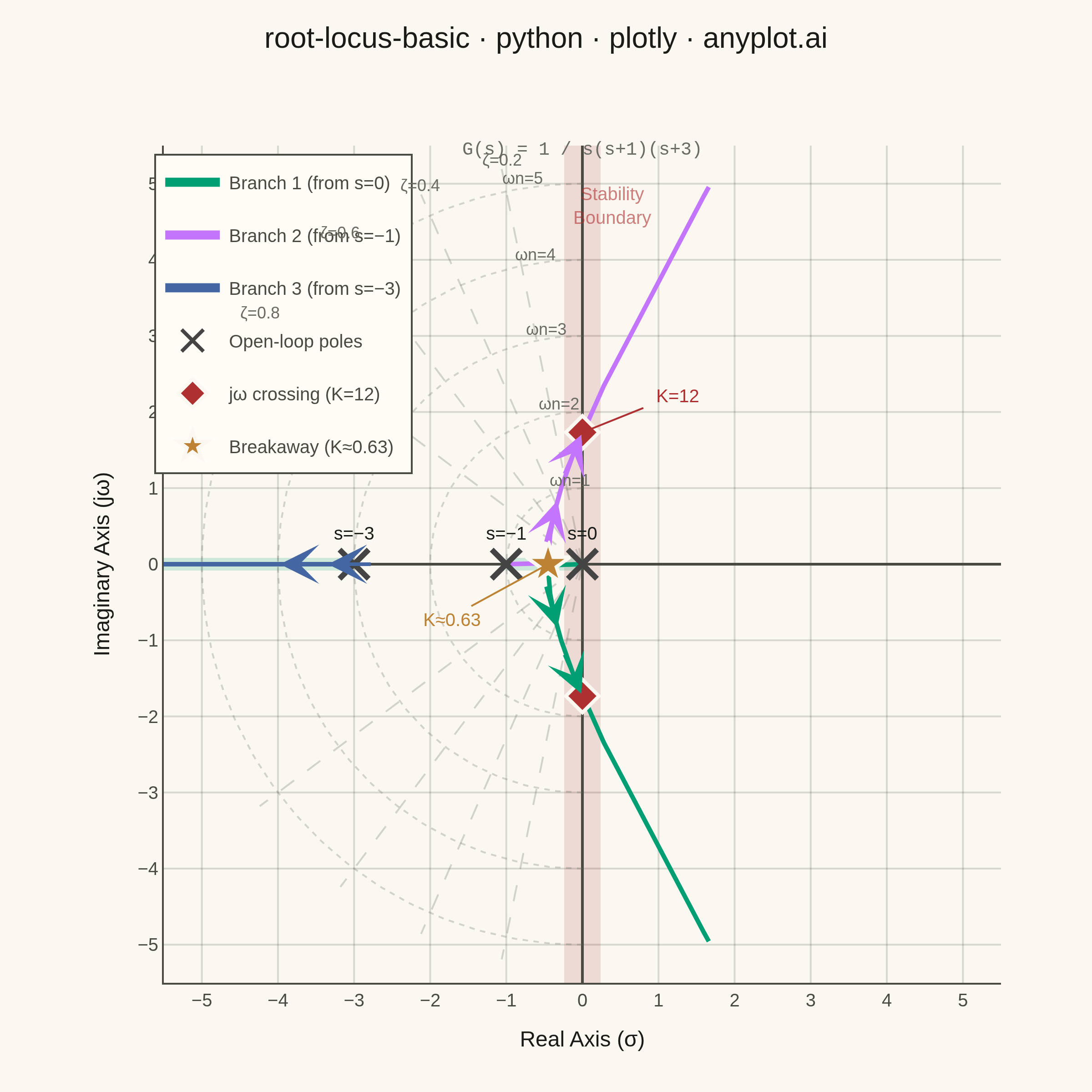
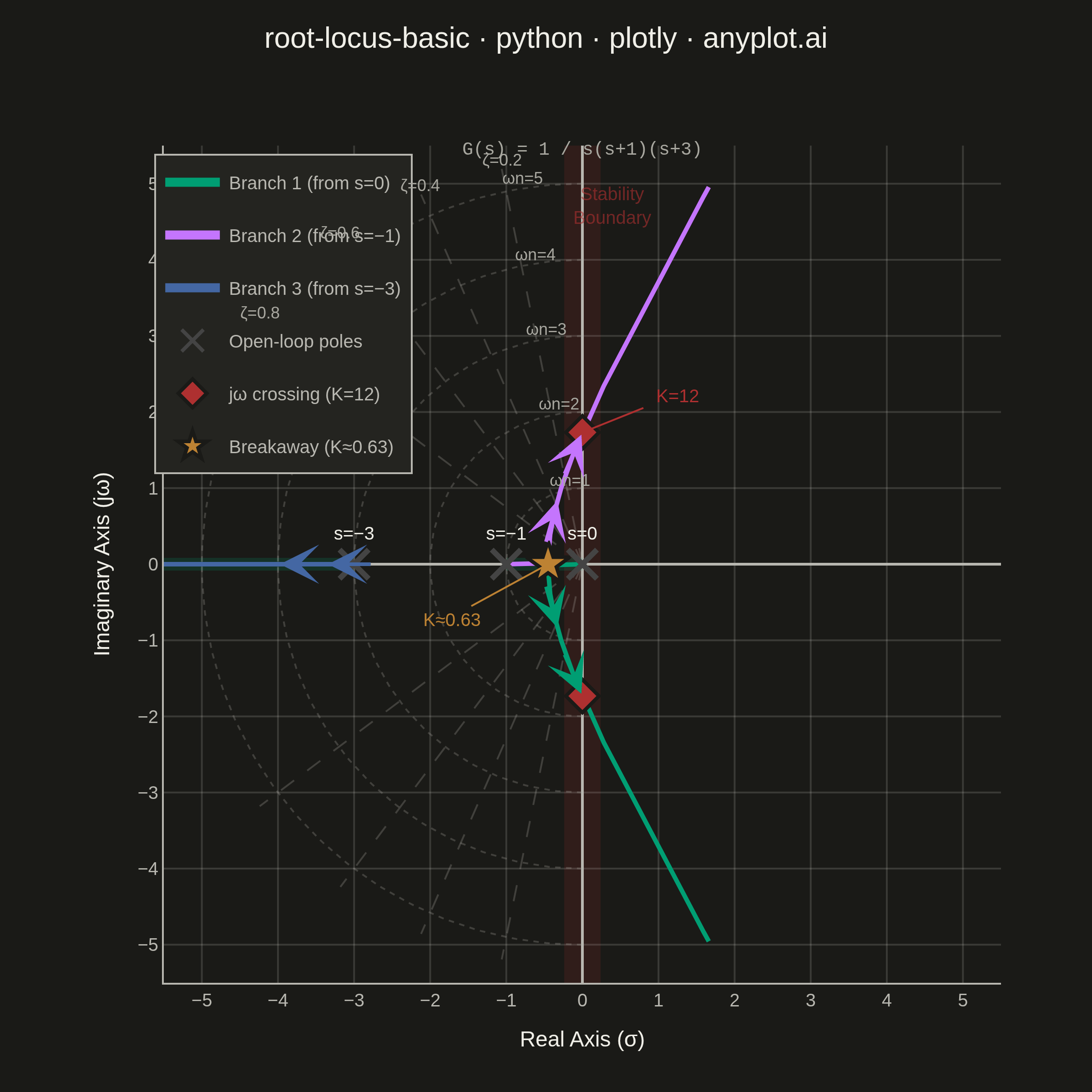
A root locus plot traces how the closed-loop poles of a transfer function migrate through the complex plane as a system parameter (typically gain K) varies from 0 to infinity. It is a fundamental tool in classical control theory for analyzing system stability and designing controllers. The plot reveals critical information about pole trajectories, stability boundaries, and gain margins.
""" anyplot.ai
root-locus-basic: Root Locus Plot for Control Systems
Library: plotly 6.8.0 | Python 3.13.14
Quality: 86/100 | Updated: 2026-06-18
"""

import os

import numpy as np
import plotly.graph_objects as go


# Theme tokens — Imprint palette, theme-adaptive chrome
THEME = os.getenv("ANYPLOT_THEME", "light")
PAGE_BG = "#FAF8F1" if THEME == "light" else "#1A1A17"
ELEVATED_BG = "#FFFDF6" if THEME == "light" else "#242420"
INK = "#1A1A17" if THEME == "light" else "#F0EFE8"
INK_SOFT = "#4A4A44" if THEME == "light" else "#B8B7B0"
INK_MUTED = "#6B6A63" if THEME == "light" else "#A8A79F"
GRID = "rgba(26,26,23,0.15)" if THEME == "light" else "rgba(240,239,232,0.15)"
REF_LINE = "rgba(107,106,99,0.28)" if THEME == "light" else "rgba(168,167,159,0.28)"

# Imprint categorical palette — positions 1–3 for the three root locus branches
BRANCH_COLORS = ["#009E73", "#C475FD", "#4467A3"]

# Data: G(s) = 1 / (s(s+1)(s+3))
# Open-loop poles at s = 0, -1, -3; no finite zeros
# Characteristic equation: s^3 + 4s^2 + 3s + K = 0
open_loop_poles = np.array([0.0, -1.0, -3.0])

gains = np.concatenate(
    [
        np.linspace(0, 0.5, 200),
        np.linspace(0.5, 4, 400),
        np.linspace(4, 12, 400),
        np.linspace(12, 50, 300),
        np.linspace(50, 200, 200),
    ]
)

branches = {i: {"real": [], "imag": [], "gain": []} for i in range(3)}
prev_roots = open_loop_poles.copy().astype(complex)

for K in gains:
    roots = np.roots([1, 4, 3, K])
    roots = np.sort_complex(roots)
    used = [False] * 3
    assignment = [0] * 3
    for i in range(3):
        best_j, best_dist = -1, np.inf
        for j in range(3):
            if not used[j]:
                d = abs(prev_roots[i] - roots[j])
                if d < best_dist:
                    best_dist = d
                    best_j = j
        used[best_j] = True
        assignment[i] = best_j
    for i in range(3):
        r = roots[assignment[i]]
        branches[i]["real"].append(r.real)
        branches[i]["imag"].append(r.imag)
        branches[i]["gain"].append(K)
    prev_roots = np.array([roots[assignment[i]] for i in range(3)])

branch_names = ["Branch 1 (from s=0)", "Branch 2 (from s=−1)", "Branch 3 (from s=−3)"]

# Plot
fig = go.Figure()

# Real axis root locus segments: [−1, 0] and (−∞, −3]
for seg in [[-1, 0], [-5.5, -3]]:
    fig.add_trace(
        go.Scatter(
            x=seg,
            y=[0, 0],
            mode="lines",
            line={"width": 7, "color": "rgba(0,158,115,0.18)"},
            showlegend=False,
            hoverinfo="skip",
        )
    )

# Constant damping ratio lines (ζ = 0.2, 0.4, 0.6, 0.8)
r_max = 5.3
for zeta in [0.2, 0.4, 0.6, 0.8]:
    r_line = np.linspace(0, r_max, 2)
    x_vals = -r_line * zeta
    y_vals = r_line * np.sqrt(1 - zeta**2)
    for sign in [1, -1]:
        fig.add_trace(
            go.Scatter(
                x=x_vals,
                y=sign * y_vals,
                mode="lines",
                line={"width": 1, "color": REF_LINE, "dash": "dash"},
                showlegend=False,
                hoverinfo="skip",
            )
        )
    fig.add_annotation(
        x=x_vals[-1], y=y_vals[-1] + 0.12, text=f"ζ={zeta}", showarrow=False, font={"size": 10, "color": INK_MUTED}
    )

# Constant natural frequency arcs (ωn = 1, 2, 3, 4, 5)
theta = np.linspace(np.pi / 2, np.pi, 100)
for wn in [1, 2, 3, 4, 5]:
    for sign in [1, -1]:
        fig.add_trace(
            go.Scatter(
                x=wn * np.cos(theta),
                y=sign * wn * np.sin(theta),
                mode="lines",
                line={"width": 1, "color": REF_LINE, "dash": "dot"},
                showlegend=False,
                hoverinfo="skip",
            )
        )
    fig.add_annotation(
        x=wn * np.cos(np.pi * 0.55),
        y=wn * np.sin(np.pi * 0.55) + 0.12,
        text=f"ωn={wn}",
        showarrow=False,
        font={"size": 10, "color": INK_MUTED},
    )

# Stability boundary — imaginary axis shaded band
fig.add_shape(
    type="line", x0=0, x1=0, y0=-5.5, y1=5.5, line={"color": "rgba(174,48,48,0.15)", "width": 20}, layer="below"
)
fig.add_annotation(
    x=0.4,
    y=4.7,
    text="Stability<br>Boundary",
    showarrow=False,
    font={"size": 10, "color": "rgba(174,48,48,0.6)", "family": "Arial, sans-serif"},
)

# Root locus branches
for i in range(3):
    fig.add_trace(
        go.Scatter(
            x=branches[i]["real"],
            y=branches[i]["imag"],
            mode="lines",
            line={"width": 2.5, "color": BRANCH_COLORS[i]},
            name=branch_names[i],
            legendgroup=f"branch{i}",
            hovertemplate=(
                f"<b>Branch {i + 1}</b><br>σ = %{{x:.3f}}<br>jω = %{{y:.3f}}<br>K = %{{customdata:.2f}}<extra></extra>"
            ),
            customdata=branches[i]["gain"],
        )
    )

# Direction arrows indicating increasing gain
for i in range(3):
    n = len(branches[i]["real"])
    for frac in [0.3, 0.65]:
        idx = int(n * frac)
        if idx < n - 5:
            dx = branches[i]["real"][idx + 5] - branches[i]["real"][idx]
            dy = branches[i]["imag"][idx + 5] - branches[i]["imag"][idx]
            norm = np.sqrt(dx**2 + dy**2)
            if norm > 1e-6:
                fig.add_annotation(
                    x=branches[i]["real"][idx],
                    y=branches[i]["imag"][idx],
                    ax=-dx / norm * 25,
                    ay=dy / norm * 25,
                    xref="x",
                    yref="y",
                    axref="pixel",
                    ayref="pixel",
                    showarrow=True,
                    arrowhead=3,
                    arrowsize=1.8,
                    arrowwidth=2,
                    arrowcolor=BRANCH_COLORS[i],
                    text="",
                )

# Open-loop poles (× markers)
fig.add_trace(
    go.Scatter(
        x=open_loop_poles,
        y=np.zeros(3),
        mode="markers+text",
        marker={"symbol": "x-thin", "size": 16, "color": INK, "line": {"width": 3}},
        text=["s=0", "s=−1", "s=−3"],
        textposition="top center",
        textfont={"size": 10, "color": INK},
        name="Open-loop poles",
        hovertemplate="Pole at s = %{x:.1f}<extra></extra>",
    )
)

# jω-axis crossing (Routh–Hurwitz: K_crit = 12, roots at ±j√3)
K_crit = 12.0
jw_cross = np.sqrt(3)
fig.add_trace(
    go.Scatter(
        x=[0, 0],
        y=[jw_cross, -jw_cross],
        mode="markers",
        marker={"symbol": "diamond", "size": 14, "color": "#AE3030", "line": {"width": 2, "color": PAGE_BG}},
        name=f"jω crossing (K={K_crit:.0f})",
        hovertemplate="s = %{y:+.3f}j<br>K = 12 (critical gain)<extra></extra>",
    )
)
fig.add_annotation(
    x=0,
    y=jw_cross,
    text=f"  K={K_crit:.0f}",
    showarrow=True,
    arrowhead=0,
    arrowwidth=1,
    arrowcolor="#AE3030",
    ax=50,
    ay=-20,
    font={"size": 10, "color": "#AE3030"},
)

# Breakaway point (σ ≈ −0.451)
s_break = -0.451
K_break = -(s_break**3 + 4 * s_break**2 + 3 * s_break)
fig.add_trace(
    go.Scatter(
        x=[s_break],
        y=[0],
        mode="markers",
        marker={"symbol": "star", "size": 18, "color": "#BD8233", "line": {"width": 2, "color": PAGE_BG}},
        name=f"Breakaway (K≈{K_break:.2f})",
        hovertemplate="Breakaway point<br>s ≈ −0.451<br>K ≈ %{customdata:.2f}<extra></extra>",
        customdata=[K_break],
    )
)
fig.add_annotation(
    x=s_break,
    y=0,
    text=f"  K≈{K_break:.2f}",
    showarrow=True,
    arrowhead=0,
    arrowwidth=1,
    arrowcolor="#BD8233",
    ax=-55,
    ay=30,
    font={"size": 10, "color": "#BD8233"},
)

# Layout — square canvas preserves equal axis scaling for the complex plane
axis_range = 5.5
fig.update_layout(
    autosize=False,
    title={
        "text": "root-locus-basic · python · plotly · anyplot.ai",
        "font": {"size": 16, "color": INK, "family": "Arial, sans-serif"},
        "x": 0.5,
        "xanchor": "center",
        "y": 0.975,
    },
    xaxis={
        "title": {
            "text": "Real Axis (σ)",
            "font": {"size": 12, "color": INK, "family": "Arial, sans-serif"},
            "standoff": 12,
        },
        "tickfont": {"size": 10, "color": INK_SOFT},
        "zeroline": True,
        "zerolinewidth": 1.5,
        "zerolinecolor": INK_SOFT,
        "showgrid": True,
        "gridwidth": 1,
        "gridcolor": GRID,
        "range": [-axis_range, axis_range],
        "constrain": "domain",
        "dtick": 1,
        "linecolor": INK_SOFT,
    },
    yaxis={
        "title": {
            "text": "Imaginary Axis (jω)",
            "font": {"size": 12, "color": INK, "family": "Arial, sans-serif"},
            "standoff": 12,
        },
        "tickfont": {"size": 10, "color": INK_SOFT},
        "zeroline": True,
        "zerolinewidth": 1.5,
        "zerolinecolor": INK_SOFT,
        "showgrid": True,
        "gridwidth": 1,
        "gridcolor": GRID,
        "range": [-axis_range, axis_range],
        "scaleanchor": "x",
        "scaleratio": 1,
        "dtick": 1,
        "linecolor": INK_SOFT,
    },
    paper_bgcolor=PAGE_BG,
    plot_bgcolor=PAGE_BG,
    font={"color": INK},
    legend={
        "font": {"size": 10, "color": INK_SOFT, "family": "Arial, sans-serif"},
        "bgcolor": ELEVATED_BG,
        "bordercolor": INK_SOFT,
        "borderwidth": 1,
        "x": 0.99,
        "y": 0.01,
        "xanchor": "right",
        "yanchor": "bottom",
        "itemsizing": "constant",
    },
    margin={"l": 80, "r": 40, "t": 80, "b": 60},
    hoverlabel={"bgcolor": ELEVATED_BG, "font_size": 12, "bordercolor": INK_SOFT},
)

# Transfer function subtitle — lower-left, clear of legend (lower-right) and ζ labels (upper-left)
fig.add_annotation(
    text="G(s) = 1 / s(s+1)(s+3)",
    xref="paper",
    yref="paper",
    x=0.03,
    y=0.03,
    xanchor="left",
    yanchor="bottom",
    showarrow=False,
    font={"size": 10, "color": INK_MUTED, "family": "Courier New, monospace"},
)

# Save — square canvas (2400×2400)
fig.write_image(f"plot-{THEME}.png", width=600, height=600, scale=4)
fig.write_html(f"plot-{THEME}.html", include_plotlyjs="cdn")
Runnable source as JSON, for any HTTP client: https://api.anyplot.ai/specs/root-locus-basic/plotly/code. Any spec id and library id listed in llms-full.txt fit the same URL shape; every URL below is complete and callable.
{
  "spec_id": "root-locus-basic",
  "language": "python",
  "library": "plotly",
  "page": "https://anyplot.ai/root-locus-basic/python/plotly",
  "hub": "https://anyplot.ai/root-locus-basic",
  "code_json": "https://api.anyplot.ai/specs/root-locus-basic/plotly/code",
  "spec_json": "https://api.anyplot.ai/specs/root-locus-basic",
  "render_light_png": "https://storage.googleapis.com/anyplot-images/plots/root-locus-basic/python/plotly/plot-light.png",
  "render_dark_png": "https://storage.googleapis.com/anyplot-images/plots/root-locus-basic/python/plotly/plot-dark.png",
  "interactive_light_html": "https://storage.googleapis.com/anyplot-images/plots/root-locus-basic/python/plotly/plot-light.html",
  "interactive_dark_html": "https://storage.googleapis.com/anyplot-images/plots/root-locus-basic/python/plotly/plot-dark.html",
  "quality_score": 86.0,
  "license": "MIT",
  "guide": "https://anyplot.ai/llms.txt"
}
Part of Root Locus Plot for Control Systems on anyplot.ai.