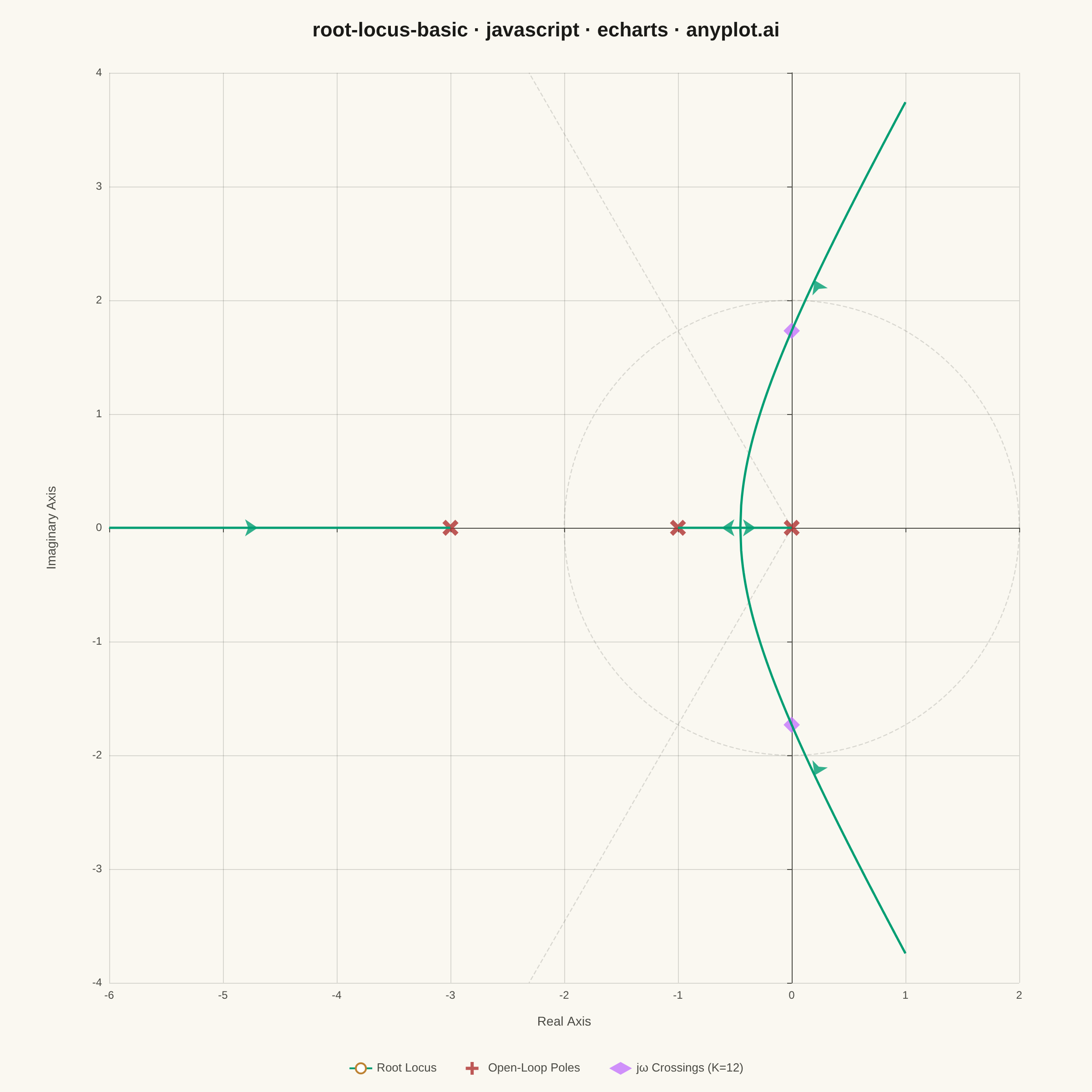
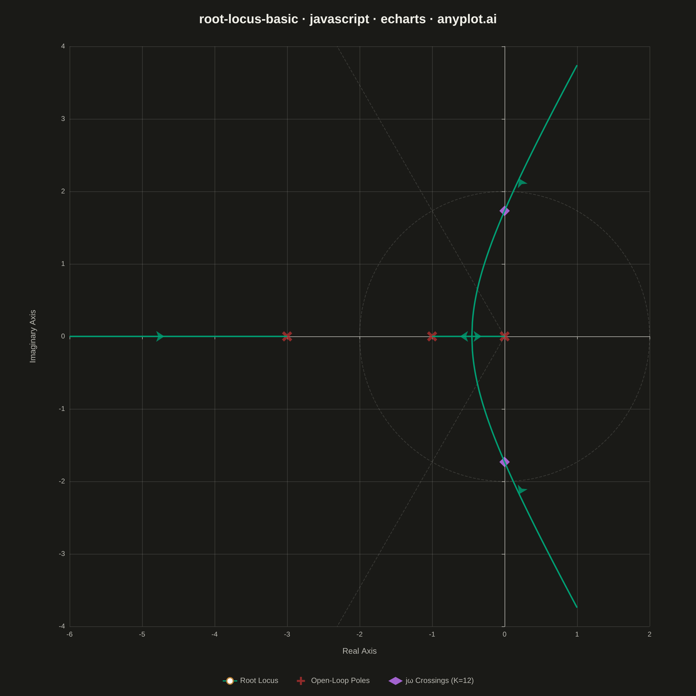
A root locus plot traces how the closed-loop poles of a transfer function migrate through the complex plane as a system parameter (typically gain K) varies from 0 to infinity. It is a fundamental tool in classical control theory for analyzing system stability and designing controllers. The plot reveals critical information about pole trajectories, stability boundaries, and gain margins.
// anyplot.ai
// root-locus-basic: Root Locus Plot for Control Systems
// Library: echarts 5.5.1 | JavaScript 22.22.3
// Quality: 84/100 | Created: 2026-06-18
//# anyplot-orientation: square
// anyplot.ai
// root-locus-basic: Root Locus Plot for Control Systems
// Library: echarts 5.5.1 | JavaScript 22.22.3
// Quality: 78/100 | Created: 2026-06-18

const t = window.ANYPLOT_TOKENS;

// Open-loop: G(s) = K / [s(s+1)(s+3)] — poles {0, −1, −3}, no zeros
// Char eq: s³ + 4s² + 3s + K = 0
// Real-axis locus: (−∞, −3] ∪ [−1, 0]  |  Breakaway: s ≈ −0.4514 at K ≈ 0.631
// jω crossing: s = ±j√3 at K = 12  |  Asymptotes: 60°, 180°, 300° from (−4/3, 0)

// Parametric formulas for complex conjugate pair given real root σ_C (Vieta):
//   σ_AB = (−4 − σ_C)/2,   ω² = 3 − σ_AB² − 2·σ_C·σ_AB
function cplxPair(sigC) {
  const sig = (-4 - sigC) / 2;
  const omegaSq = 3 - sig * sig - 2 * sigC * sig;
  return { sig, omega: Math.sqrt(Math.max(0, omegaSq)) };
}

const BKWY = -0.4514;    // breakaway real coordinate
const SIG_C0 = -3.0972; // real root (branch C) at start of complex phase

// Locus path arrays: [real, imag] pairs
const bA = [], bB = [], bC = [];

// Phase 1: real-axis convergence toward breakaway (K: 0 → 0.631)
const N1 = 60;
for (let i = 0; i <= N1; i++) {
  const f = i / N1;
  bA.push([BKWY * f, 0]);                 // pole 0  → breakaway
  bB.push([-1 + 0.5486 * f, 0]);          // pole −1 → breakaway
  bC.push([-3 + (SIG_C0 + 3) * f, 0]);   // pole −3 → SIG_C0
}

// Phase 2: complex locus (K > 0.631), σ_C from SIG_C0 to −6
const N2 = 200;
for (let i = 1; i <= N2; i++) {
  const f = i / N2;
  const sigC = SIG_C0 + (-6 - SIG_C0) * f;
  const { sig, omega } = cplxPair(sigC);
  bA.push([sig, omega]);
  bB.push([sig, -omega]);
  bC.push([sigC, 0]);
}

// Constant damping-ratio reference lines: ζ = 0.5 (angle 60° from −Re axis)
// Direction: (cos 120°, ±sin 120°) = (−0.5, ±√3/2)
// Exits at y = ±4 when r = 4/(√3/2) ≈ 4.619, x = −4.619×0.5 ≈ −2.309
const zeta05up = [[0, 0], [-2.309, 4]];
const zeta05dn = [[0, 0], [-2.309, -4]];

// Natural frequency reference circle: ωn = 2 (full circle, r = 2)
const wnCircle = [];
for (let i = 0; i <= 360; i++) {
  const theta = (i / 180) * Math.PI;
  wnCircle.push([2 * Math.cos(theta), 2 * Math.sin(theta)]);
}

// Key markers
const poles = [[0, 0], [-1, 0], [-3, 0]];
const jwCross = [[0, Math.sqrt(3)], [0, -Math.sqrt(3)]]; // ±j√3, K=12

// Gain-direction arrows: symbolRotate = atan2(dx, dy) maps chart tangent to
// ECharts clockwise-from-up convention (right→90°, up→0°, left→-90°, down→180°)
function arrowAt(path, idx) {
  const i = Math.max(1, Math.min(path.length - 2, idx));
  const dx = path[i + 1][0] - path[i - 1][0];
  const dy = path[i + 1][1] - path[i - 1][1];
  return { value: path[i], symbolRotate: Math.atan2(dx, dy) * 180 / Math.PI };
}

const gainArrows = [
  arrowAt(bA, Math.floor(N1 * 0.70)),        // phase 1, bA: leftward (K↑ toward breakaway)
  arrowAt(bB, Math.floor(N1 * 0.70)),        // phase 1, bB: rightward (K↑ toward breakaway)
  arrowAt(bA, N1 + Math.floor(N2 * 0.45)),   // phase 2, bA: upper-right (K↑ along complex branch)
  arrowAt(bB, N1 + Math.floor(N2 * 0.45)),   // phase 2, bB: lower-right (K↑ along complex branch)
  arrowAt(bC, N1 + Math.floor(N2 * 0.55)),   // phase 2, bC: leftward (K↑ along real branch)
];

// ── Chart ─────────────────────────────────────────────────────────────────────
const chart = echarts.init(document.getElementById("container"));

chart.setOption({
  animation: false,
  color: t.palette,
  backgroundColor: "transparent",

  title: {
    text: "root-locus-basic · javascript · echarts · anyplot.ai",
    left: "center",
    top: 18,
    textStyle: { color: t.ink, fontSize: 22, fontWeight: "bold" },
  },

  legend: {
    bottom: 14,
    itemGap: 32,
    textStyle: { color: t.inkSoft, fontSize: 13 },
  },

  // Square grid (2200×2200 within 2400×2400 canvas) for equal axis scaling:
  // x range 8 units and y range 8 units → 275 px/unit on each axis
  grid: { left: 120, right: 80, top: 80, bottom: 120 },

  xAxis: {
    type: "value",
    name: "Real Axis",
    nameLocation: "middle",
    nameGap: 36,
    nameTextStyle: { color: t.inkSoft, fontSize: 14 },
    min: -6,
    max: 2,
    interval: 1,
    axisLabel: { color: t.inkSoft, fontSize: 12 },
    axisLine: { show: true, lineStyle: { color: t.inkSoft } },
    axisTick: { show: true, lineStyle: { color: t.inkSoft } },
    splitLine: { lineStyle: { color: t.grid, width: 1 } },
  },

  yAxis: {
    type: "value",
    name: "Imaginary Axis",
    nameLocation: "middle",
    nameGap: 56,
    nameTextStyle: { color: t.inkSoft, fontSize: 14 },
    min: -4,
    max: 4,
    interval: 1,
    axisLabel: { color: t.inkSoft, fontSize: 12 },
    axisLine: { show: true, lineStyle: { color: t.inkSoft } },
    axisTick: { show: true, lineStyle: { color: t.inkSoft } },
    splitLine: { lineStyle: { color: t.grid, width: 1 } },
  },

  series: [
    // ζ = 0.5 damping-ratio reference lines (subtle dashed, excluded from legend)
    {
      type: "line",
      data: zeta05up,
      showSymbol: false,
      lineStyle: { color: t.grid, width: 1.2, type: "dashed" },
      silent: true,
      legendHoverLink: false,
    },
    {
      type: "line",
      data: zeta05dn,
      showSymbol: false,
      lineStyle: { color: t.grid, width: 1.2, type: "dashed" },
      silent: true,
      legendHoverLink: false,
    },
    // ωn = 2 natural frequency reference circle (now renders as true circle)
    {
      type: "line",
      data: wnCircle,
      showSymbol: false,
      lineStyle: { color: t.grid, width: 1.2, type: "dashed" },
      silent: true,
      legendHoverLink: false,
    },
    // Root locus branches (A upper, B lower, C real — share one legend entry)
    {
      name: "Root Locus",
      type: "line",
      data: bA,
      showSymbol: false,
      lineStyle: { color: t.palette[0], width: 2.5 },
    },
    {
      name: "Root Locus",
      type: "line",
      data: bB,
      showSymbol: false,
      lineStyle: { color: t.palette[0], width: 2.5 },
    },
    {
      name: "Root Locus",
      type: "line",
      data: bC,
      showSymbol: false,
      lineStyle: { color: t.palette[0], width: 2.5 },
    },
    // Gain-direction arrows (excluded from legend — decorative overlay)
    {
      type: "scatter",
      data: gainArrows,
      symbol: "arrow",
      symbolSize: 14,
      itemStyle: { color: t.palette[0] },
      silent: true,
      legendHoverLink: false,
    },
    // Open-loop poles (× markers via rotated cross shape)
    {
      name: "Open-Loop Poles",
      type: "scatter",
      data: poles,
      symbol:
        "path://M-1,-4 L1,-4 L1,-1 L4,-1 L4,1 L1,1 L1,4 L-1,4 L-1,1 L-4,1 L-4,-1 L-1,-1 Z",
      symbolSize: 20,
      symbolRotate: 45,
      itemStyle: { color: t.palette[4] },
    },
    // Stability boundary crossings ±j√3 at K = 12
    {
      name: "jω Crossings (K=12)",
      type: "scatter",
      data: jwCross,
      symbol: "diamond",
      symbolSize: 18,
      itemStyle: { color: t.palette[1] },
    },
  ],
});
Runnable source as JSON, for any HTTP client: https://api.anyplot.ai/specs/root-locus-basic/echarts/code. Any spec id and library id listed in llms-full.txt fit the same URL shape; every URL below is complete and callable.
{
  "spec_id": "root-locus-basic",
  "language": "javascript",
  "library": "echarts",
  "page": "https://anyplot.ai/root-locus-basic/javascript/echarts",
  "hub": "https://anyplot.ai/root-locus-basic",
  "code_json": "https://api.anyplot.ai/specs/root-locus-basic/echarts/code",
  "spec_json": "https://api.anyplot.ai/specs/root-locus-basic",
  "render_light_png": "https://storage.googleapis.com/anyplot-images/plots/root-locus-basic/javascript/echarts/plot-light.png",
  "render_dark_png": "https://storage.googleapis.com/anyplot-images/plots/root-locus-basic/javascript/echarts/plot-dark.png",
  "interactive_light_html": "https://storage.googleapis.com/anyplot-images/plots/root-locus-basic/javascript/echarts/plot-light.html",
  "interactive_dark_html": "https://storage.googleapis.com/anyplot-images/plots/root-locus-basic/javascript/echarts/plot-dark.html",
  "quality_score": 84.0,
  "license": "MIT",
  "guide": "https://anyplot.ai/llms.txt"
}
Part of Root Locus Plot for Control Systems on anyplot.ai.