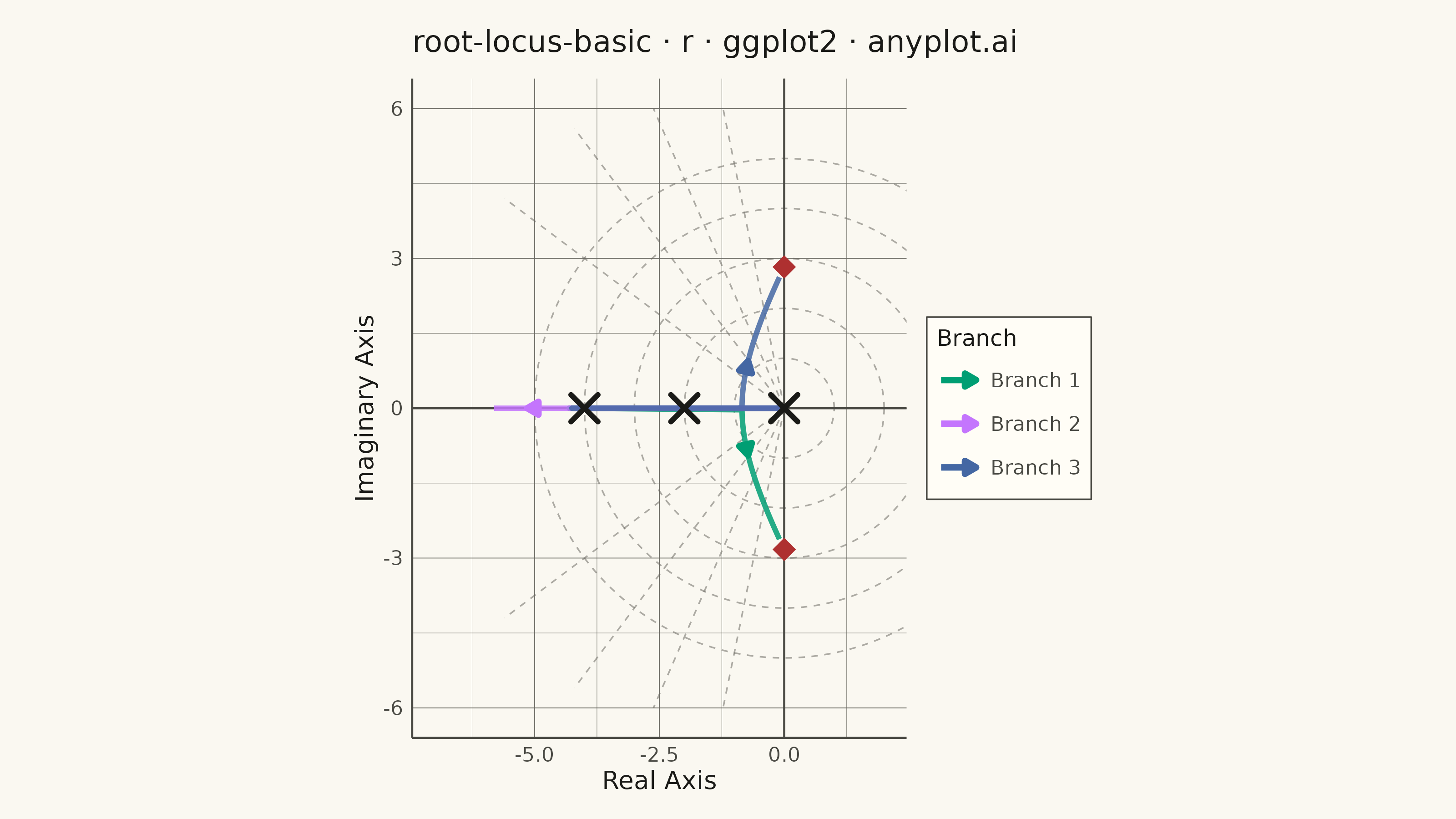
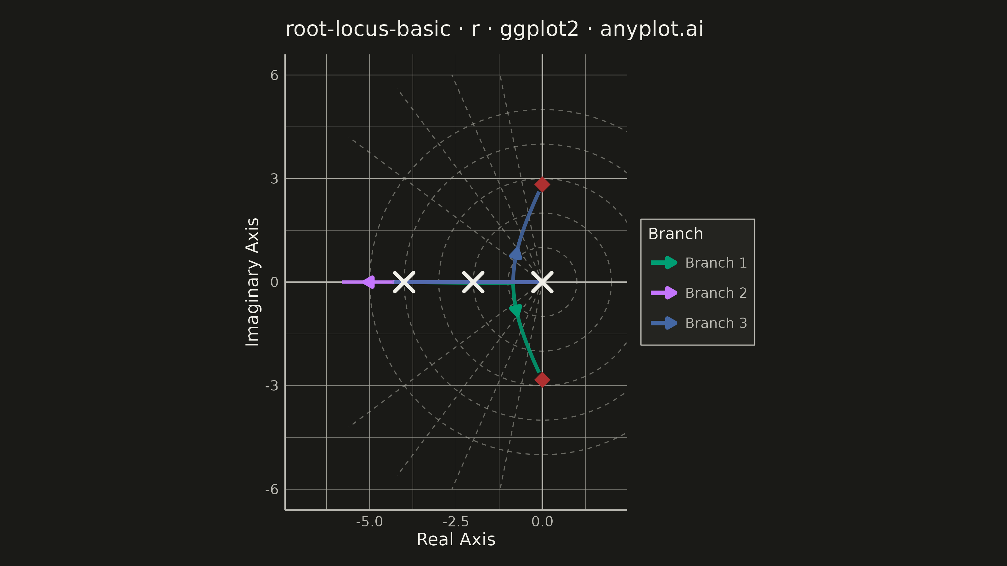
A root locus plot traces how the closed-loop poles of a transfer function migrate through the complex plane as a system parameter (typically gain K) varies from 0 to infinity. It is a fundamental tool in classical control theory for analyzing system stability and designing controllers. The plot reveals critical information about pole trajectories, stability boundaries, and gain margins.
#' anyplot.ai
#' root-locus-basic: Root Locus Plot for Control Systems
#' Library: ggplot2 3.5.1 | R 4.4.1
#' Quality: 86/100 | Created: 2026-06-18

library(ggplot2)
library(dplyr)
library(ragg)

set.seed(42)

# Theme tokens
THEME       <- Sys.getenv("ANYPLOT_THEME", "light")
PAGE_BG     <- if (THEME == "light") "#FAF8F1" else "#1A1A17"
ELEVATED_BG <- if (THEME == "light") "#FFFDF6" else "#242420"
INK         <- if (THEME == "light") "#1A1A17" else "#F0EFE8"
INK_SOFT    <- if (THEME == "light") "#4A4A44" else "#B8B7B0"
INK_MUTED   <- if (THEME == "light") "#6B6A63" else "#A8A79F"

IMPRINT_PALETTE <- c(
  "#009E73",  # 1 — brand green
  "#C475FD",  # 2 — lavender
  "#4467A3",  # 3 — blue
  "#BD8233",  # 4 — ochre
  "#AE3030"   # 5 — matte red
)

# Data: third-order system  G(s) = K / (s(s+2)(s+4))
# Open-loop poles: 0, -2, -4. No finite zeros.
# Root locus computed numerically by sweeping K.
gain_vals <- c(seq(0, 2, length.out = 300),
               seq(2, 10, length.out = 400),
               seq(10, 40, length.out = 300))
gain_vals <- sort(unique(gain_vals))

# Characteristic polynomial: s^3 + 6s^2 + 8s + K = 0
# Roots via polyroot for each K
root_locus_rows <- lapply(gain_vals, function(K) {
  # coefficients: s^3 + 6s^2 + 8s + K
  r <- polyroot(c(K, 8, 6, 1))
  # Sort by imaginary part to keep branch assignment consistent
  r <- r[order(Im(r))]
  list(
    gain   = rep(K, 3),
    branch = c("Branch 1", "Branch 2", "Branch 3"),
    re     = Re(r),
    im     = Im(r)
  )
})

df <- bind_rows(lapply(root_locus_rows, function(x) {
  data.frame(gain = x$gain, branch = x$branch, re = x$re, im = x$im,
             stringsAsFactors = FALSE)
}))

# Keep only points within a reasonable window
df <- df[abs(df$re) <= 8 & abs(df$im) <= 8, ]

# Open-loop poles (K=0)
poles <- data.frame(re = c(0, -2, -4), im = c(0, 0, 0))

# Imaginary axis crossing: K at which Routh criterion gives jw roots
# For s^3+6s^2+8s+K: Routh row 1=[1,8], row 2=[6,K], pivot=(48-K)/6
# Crossing when K=48, auxiliary eq 6s^2+48=0 -> s=+/-j*sqrt(8)
crossing <- data.frame(re = c(0, 0), im = c(sqrt(8), -sqrt(8)))

# Arrow data: show direction of increasing gain along each branch
arrow_k_vals <- c(6, 18, 6)  # one per branch at a distinctive location
branch_names <- c("Branch 1", "Branch 2", "Branch 3")

arrow_df <- bind_rows(lapply(seq_along(branch_names), function(i) {
  k0 <- arrow_k_vals[i]
  dk <- 0.6
  seg_start <- df[abs(df$gain - k0) < 0.15 & df$branch == branch_names[i], ][1, ]
  seg_end   <- df[abs(df$gain - (k0 + dk)) < 0.15 & df$branch == branch_names[i], ][1, ]
  if (!is.na(seg_start$re) && !is.na(seg_end$re)) {
    data.frame(x = seg_start$re, y = seg_start$im,
               xend = seg_end$re, yend = seg_end$im,
               branch = branch_names[i])
  }
}))

# Damping ratio reference lines: radial rays from origin at angle arccos(zeta)
# from the negative real axis. A pole with damping ratio zeta lies at angle
# (pi - arccos(zeta)) from the positive real axis => direction (-zeta, sqrt(1-zeta^2)).
zeta_vals <- c(0.2, 0.4, 0.6, 0.8)
plot_re_max <- 7
plot_im_max <- 6

zeta_df <- bind_rows(lapply(zeta_vals, function(z) {
  re_end <- -plot_re_max * z
  im_end <- plot_re_max * sqrt(1 - z^2)
  # Clip to plot bounds
  if (abs(im_end) > plot_im_max) {
    sc <- plot_im_max / abs(im_end)
    re_end <- re_end * sc
    im_end <- im_end * sc
  }
  rbind(
    data.frame(x = 0, y = 0, xend = re_end, yend =  im_end),
    data.frame(x = 0, y = 0, xend = re_end, yend = -im_end)
  )
}))

# Natural frequency circles: concentric circles at omega_n = 1..5
omega_df <- bind_rows(lapply(1:5, function(w) {
  theta <- seq(0, 2 * pi, length.out = 200)
  data.frame(re = w * cos(theta), im = w * sin(theta), grp = paste0("wn", w))
}))

# Title
plot_title <- "root-locus-basic · r · ggplot2 · anyplot.ai"
title_size <- 12

# Plot
p <- ggplot(df, aes(x = re, y = im, color = branch, group = branch)) +
  # Natural frequency circles (dashed, muted — behind locus)
  geom_path(
    data = omega_df,
    aes(x = re, y = im, group = grp),
    color = INK_MUTED, linewidth = 0.3, linetype = "dashed",
    alpha = 0.55, inherit.aes = FALSE
  ) +
  # Damping ratio rays (dashed, muted — behind locus)
  geom_segment(
    data = zeta_df,
    aes(x = x, y = y, xend = xend, yend = yend),
    color = INK_MUTED, linewidth = 0.3, linetype = "dashed",
    alpha = 0.55, inherit.aes = FALSE
  ) +
  # Axis reference lines
  geom_hline(yintercept = 0, color = INK_SOFT, linewidth = 0.4) +
  geom_vline(xintercept = 0, color = INK_SOFT, linewidth = 0.4) +
  # Root locus branches
  geom_path(linewidth = 1.0, alpha = 0.85) +
  # Direction arrows
  geom_segment(
    data = arrow_df,
    aes(x = x, y = y, xend = xend, yend = yend, color = branch),
    arrow = arrow(length = unit(0.18, "cm"), type = "closed"),
    linewidth = 1.2,
    inherit.aes = FALSE
  ) +
  # Imaginary axis crossings (stability boundary)
  geom_point(
    data = crossing,
    aes(x = re, y = im),
    shape = 18, size = 4, color = IMPRINT_PALETTE[5],
    inherit.aes = FALSE
  ) +
  # Open-loop poles
  geom_point(
    data = poles,
    aes(x = re, y = im),
    shape = 4, size = 4, stroke = 1.5, color = INK,
    inherit.aes = FALSE
  ) +
  # Color scale (3 branches)
  scale_color_manual(
    values = IMPRINT_PALETTE[1:3],
    name   = "Branch"
  ) +
  # Equal axes to preserve geometry
  coord_equal(xlim = c(-7, 2), ylim = c(-6, 6)) +
  labs(
    title = plot_title,
    x     = "Real Axis",
    y     = "Imaginary Axis"
  ) +
  theme_minimal(base_size = 8) +
  theme(
    plot.background   = element_rect(fill = PAGE_BG,     color = PAGE_BG),
    panel.background  = element_rect(fill = PAGE_BG,     color = NA),
    panel.grid.major  = element_line(color = INK_MUTED,  linewidth = 0.15),
    panel.grid.minor  = element_line(color = INK_MUTED,  linewidth = 0.08),
    panel.border      = element_blank(),
    axis.line         = element_line(color = INK_SOFT,   linewidth = 0.4),
    axis.title        = element_text(color = INK,        size = 10),
    axis.text         = element_text(color = INK_SOFT,   size = 8),
    plot.title        = element_text(color = INK,        size = title_size,
                                     margin = margin(b = 8)),
    legend.background = element_rect(fill = ELEVATED_BG, color = INK_SOFT,
                                     linewidth = 0.3),
    legend.text       = element_text(color = INK_SOFT,  size = 8),
    legend.title      = element_text(color = INK,       size = 9),
    legend.position   = "right",
    plot.margin       = margin(12, 14, 10, 10)
  )

# Save
ggsave(
  filename = sprintf("plot-%s.png", THEME),
  plot     = p,
  device   = ragg::agg_png,
  width    = 8,
  height   = 4.5,
  units    = "in",
  dpi      = 400
)
Runnable source as JSON, for any HTTP client: https://api.anyplot.ai/specs/root-locus-basic/ggplot2/code. Any spec id and library id listed in llms-full.txt fit the same URL shape; every URL below is complete and callable.
{
  "spec_id": "root-locus-basic",
  "language": "r",
  "library": "ggplot2",
  "page": "https://anyplot.ai/root-locus-basic/r/ggplot2",
  "hub": "https://anyplot.ai/root-locus-basic",
  "code_json": "https://api.anyplot.ai/specs/root-locus-basic/ggplot2/code",
  "spec_json": "https://api.anyplot.ai/specs/root-locus-basic",
  "render_light_png": "https://storage.googleapis.com/anyplot-images/plots/root-locus-basic/r/ggplot2/plot-light.png",
  "render_dark_png": "https://storage.googleapis.com/anyplot-images/plots/root-locus-basic/r/ggplot2/plot-dark.png",
  "quality_score": 86.0,
  "license": "MIT",
  "guide": "https://anyplot.ai/llms.txt"
}
Part of Root Locus Plot for Control Systems on anyplot.ai.