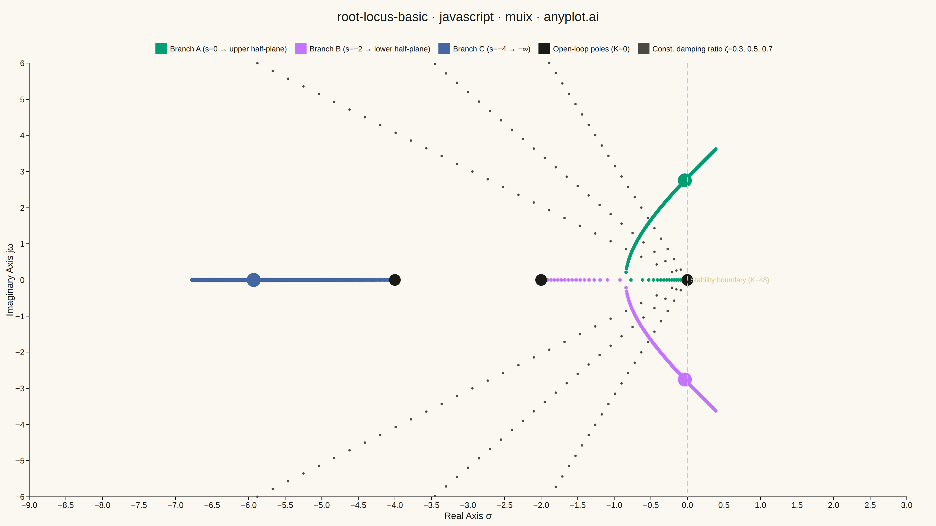
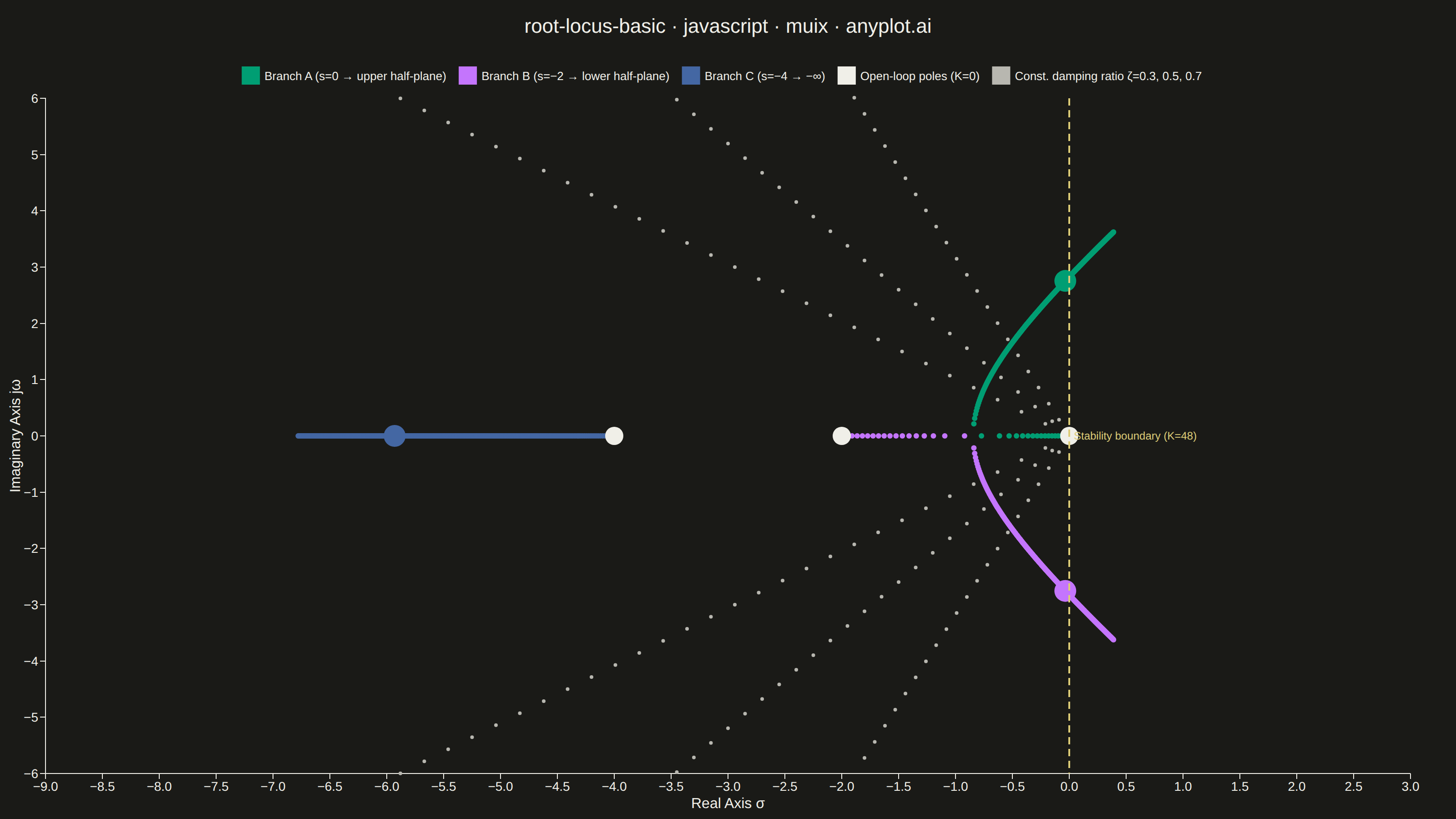
A root locus plot traces how the closed-loop poles of a transfer function migrate through the complex plane as a system parameter (typically gain K) varies from 0 to infinity. It is a fundamental tool in classical control theory for analyzing system stability and designing controllers. The plot reveals critical information about pole trajectories, stability boundaries, and gain margins.
// anyplot.ai
// root-locus-basic: Root Locus Plot for Control Systems
// Library: muix 7.29.1 | JavaScript 22.22.3
// Quality: 85/100 | Created: 2026-06-18

import { ScatterChart } from "@mui/x-charts/ScatterChart";
import { ChartsReferenceLine } from "@mui/x-charts";
import Box from "@mui/material/Box";
import Typography from "@mui/material/Typography";

const tok = window.ANYPLOT_TOKENS;

// Root locus for G(s) = K / [s(s+2)(s+4)], K ∈ [0, 90]
// Characteristic equation: s³ + 6s² + 8s + K = 0
// Open-loop poles: s = 0, −2, −4
// Breakaway at s ≈ −0.845 (K ≈ 3.08); jω crossing at K = 48 (s ≈ ±j2.83)

function polyVal(r, K) {
  return r * r * r + 6 * r * r + 8 * r + K;
}
function polyDeriv(r) {
  return 3 * r * r + 12 * r + 8;
}
function findRealRoot(K, guess) {
  let r = guess;
  for (let it = 0; it < 80; it++) {
    const fp = polyDeriv(r);
    if (Math.abs(fp) < 1e-15) break;
    const delta = polyVal(r, K) / fp;
    r -= delta;
    if (Math.abs(delta) < 1e-12) break;
  }
  return r;
}
function complexPair(r3) {
  const b = 6 + r3;
  const c = 8 + r3 * b;
  const disc = b * b - 4 * c;
  if (disc >= 0) {
    const sq = Math.sqrt(disc);
    return [{ re: (-b + sq) / 2, im: 0 }, { re: (-b - sq) / 2, im: 0 }];
  }
  const sq = Math.sqrt(-disc);
  return [{ re: -b / 2, im: sq / 2 }, { re: -b / 2, im: -sq / 2 }];
}

const N_K = 500;
const K_MAX = 90;
const branchA = [], branchB = [], branchC = [];
let r3 = -4.001;

for (let i = 0; i <= N_K; i++) {
  const K = (i / N_K) * K_MAX;
  r3 = findRealRoot(K, r3);
  const pair = complexPair(r3);
  branchA.push({ x: pair[0].re, y: pair[0].im, id: i });
  branchB.push({ x: pair[1].re, y: pair[1].im, id: i + N_K + 1 });
  branchC.push({ x: r3, y: 0, id: i + 2 * (N_K + 1) });
}

// Open-loop poles (× markers at K=0)
const poleData = [
  { x: 0, y: 0, id: 9000 },
  { x: -2, y: 0, id: 9001 },
  { x: -4, y: 0, id: 9002 },
];

// Constant damping-ratio lines: straight rays from origin for ζ = 0.3, 0.5, 0.7
// Each ray: x = -r·ζ, y = ±r·√(1−ζ²)
const dampingData = [];
let dId = 10000;
for (const zeta of [0.3, 0.5, 0.7]) {
  const sinT = Math.sqrt(1 - zeta * zeta);
  for (let k = 1; k <= 28; k++) {
    const r = k * 0.3;
    dampingData.push({ x: -r * zeta, y: r * sinT, id: dId++ });
    dampingData.push({ x: -r * zeta, y: -r * sinT, id: dId++ });
  }
}

// Gain-direction arrows at branch midpoints (K ≈ 45, index = 250)
const MID = 250;
const STEP = 15;
function dirAngle(pts) {
  const dx = pts[Math.min(MID + STEP, N_K)].x - pts[MID].x;
  const dy = pts[Math.min(MID + STEP, N_K)].y - pts[MID].y;
  return Math.atan2(dy, dx) * (180 / Math.PI);
}
const ARROW_ANGLES = {
  arrowA: dirAngle(branchA),
  arrowB: dirAngle(branchB),
  arrowC: dirAngle(branchC),
};
const arrowData = [
  { x: branchA[MID].x, y: branchA[MID].y, id: 20000 },
  { x: branchB[MID].x, y: branchB[MID].y, id: 20001 },
  { x: branchC[MID].x, y: branchC[MID].y, id: 20002 },
];

// ─── Custom mark ────────────────────────────────────────────────────────────
// × for poles, ▶ (rotated) for gain arrows, tiny dot for damping, circle otherwise
const CustomMark = ({ x, y, color, seriesId }) => {
  if (seriesId === "poles") {
    const sz = 7;
    return (
      <g>
        <line
          x1={x - sz} y1={y - sz} x2={x + sz} y2={y + sz}
          stroke={color} strokeWidth={2.5} strokeLinecap="round"
        />
        <line
          x1={x + sz} y1={y - sz} x2={x - sz} y2={y + sz}
          stroke={color} strokeWidth={2.5} strokeLinecap="round"
        />
      </g>
    );
  }
  if (seriesId in ARROW_ANGLES) {
    const angle = ARROW_ANGLES[seriesId];
    return (
      <g transform={`translate(${x},${y}) rotate(${angle})`}>
        <polygon points="-7,-5 8,0 -7,5" fill={color} opacity={0.85} />
      </g>
    );
  }
  if (seriesId === "damping") {
    return <circle cx={x} cy={y} r={1.5} fill={color} opacity={0.35} />;
  }
  return <circle cx={x} cy={y} r={2.5} fill={color} />;
};

const TITLE_H = 58;

export default function Chart() {
  return (
    <Box
      sx={{
        width: window.ANYPLOT_SIZE.width,
        height: window.ANYPLOT_SIZE.height,
        display: "flex",
        flexDirection: "column",
      }}
    >
      <Typography
        sx={{
          color: "text.primary",
          fontWeight: 500,
          fontSize: 22,
          textAlign: "center",
          lineHeight: `${TITLE_H}px`,
          height: TITLE_H,
          flexShrink: 0,
        }}
      >
        root-locus-basic · javascript · muix · anyplot.ai
      </Typography>
      <ScatterChart
        width={window.ANYPLOT_SIZE.width}
        height={window.ANYPLOT_SIZE.height - TITLE_H}
        skipAnimation
        slots={{ mark: CustomMark }}
        series={[
          {
            id: "branchA",
            label: "Branch A  (s=0 → upper half-plane)",
            data: branchA,
            color: tok.palette[0],
            markerSize: 3,
          },
          {
            id: "branchB",
            label: "Branch B  (s=−2 → lower half-plane)",
            data: branchB,
            color: tok.palette[1],
            markerSize: 3,
          },
          {
            id: "branchC",
            label: "Branch C  (s=−4 → −∞)",
            data: branchC,
            color: tok.palette[2],
            markerSize: 3,
          },
          {
            id: "poles",
            label: "Open-loop poles  (K=0)",
            data: poleData,
            color: tok.ink,
            markerSize: 10,
          },
          {
            id: "damping",
            label: "Const. damping ratio  ζ=0.3, 0.5, 0.7",
            data: dampingData,
            color: tok.inkSoft,
            markerSize: 2,
          },
          {
            id: "arrowA",
            data: [arrowData[0]],
            color: tok.palette[0],
            markerSize: 12,
          },
          {
            id: "arrowB",
            data: [arrowData[1]],
            color: tok.palette[1],
            markerSize: 12,
          },
          {
            id: "arrowC",
            data: [arrowData[2]],
            color: tok.palette[2],
            markerSize: 12,
          },
        ]}
        xAxis={[
          {
            label: "Real Axis  σ",
            min: -9,
            max: 3,
            tickLabelStyle: { fontSize: 14 },
            labelStyle: { fontSize: 16 },
          },
        ]}
        yAxis={[
          {
            label: "Imaginary Axis  jω",
            min: -6,
            max: 6,
            tickLabelStyle: { fontSize: 14 },
            labelStyle: { fontSize: 16 },
          },
        ]}
        slotProps={{
          legend: { labelStyle: { fontSize: 13 } },
        }}
      >
        <ChartsReferenceLine
          x={0}
          label="Stability boundary (K=48)"
          lineStyle={{
            stroke: tok.amber,
            strokeDasharray: "8 5",
            strokeWidth: 2,
          }}
          labelStyle={{ fontSize: 12, fill: tok.amber, dy: -10 }}
        />
      </ScatterChart>
    </Box>
  );
}
Runnable source as JSON, for any HTTP client: https://api.anyplot.ai/specs/root-locus-basic/muix/code. Any spec id and library id listed in llms-full.txt fit the same URL shape; every URL below is complete and callable.
{
  "spec_id": "root-locus-basic",
  "language": "javascript",
  "library": "muix",
  "page": "https://anyplot.ai/root-locus-basic/javascript/muix",
  "hub": "https://anyplot.ai/root-locus-basic",
  "code_json": "https://api.anyplot.ai/specs/root-locus-basic/muix/code",
  "spec_json": "https://api.anyplot.ai/specs/root-locus-basic",
  "render_light_png": "https://storage.googleapis.com/anyplot-images/plots/root-locus-basic/javascript/muix/plot-light.png",
  "render_dark_png": "https://storage.googleapis.com/anyplot-images/plots/root-locus-basic/javascript/muix/plot-dark.png",
  "interactive_light_html": "https://storage.googleapis.com/anyplot-images/plots/root-locus-basic/javascript/muix/plot-light.html",
  "interactive_dark_html": "https://storage.googleapis.com/anyplot-images/plots/root-locus-basic/javascript/muix/plot-dark.html",
  "quality_score": 85.0,
  "license": "MIT",
  "guide": "https://anyplot.ai/llms.txt"
}
Part of Root Locus Plot for Control Systems on anyplot.ai.