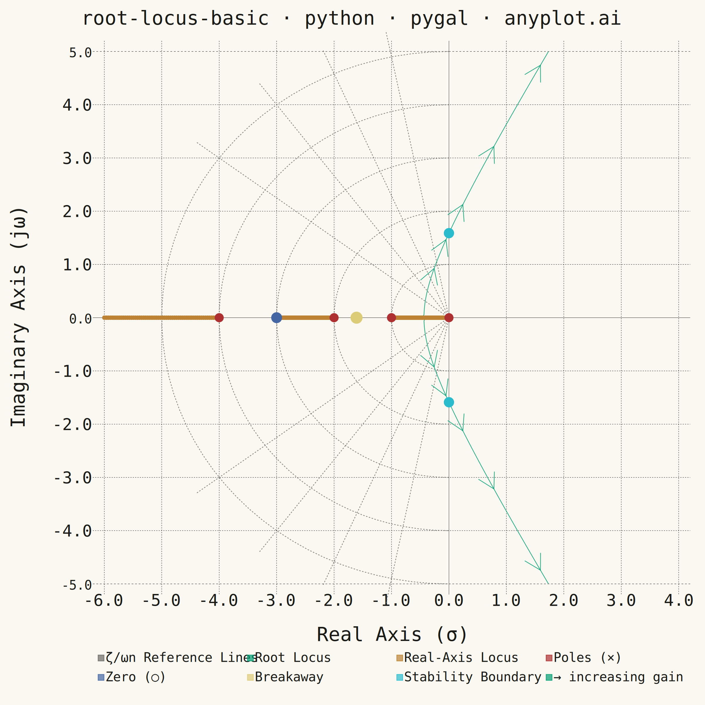
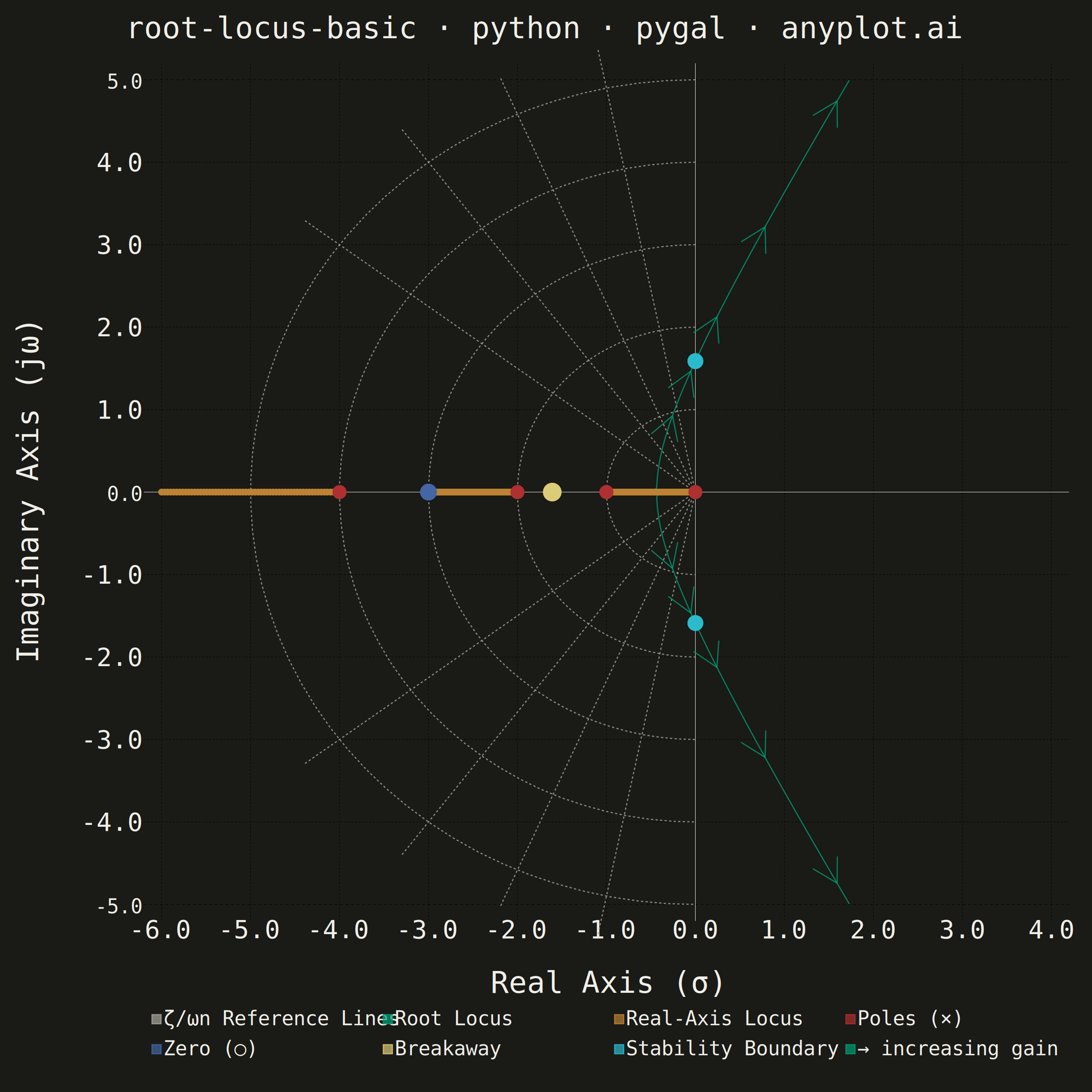
A root locus plot traces how the closed-loop poles of a transfer function migrate through the complex plane as a system parameter (typically gain K) varies from 0 to infinity. It is a fundamental tool in classical control theory for analyzing system stability and designing controllers. The plot reveals critical information about pole trajectories, stability boundaries, and gain margins.
""" anyplot.ai
root-locus-basic: Root Locus Plot for Control Systems
Library: pygal 3.1.0 | Python 3.13.13
Quality: 87/100 | Updated: 2026-06-18
"""

import os

import numpy as np
import pygal
from pygal.style import Style


# Theme tokens
THEME = os.getenv("ANYPLOT_THEME", "light")
PAGE_BG = "#FAF8F1" if THEME == "light" else "#1A1A17"
INK = "#1A1A17" if THEME == "light" else "#F0EFE8"
INK_MUTED = "#6B6A63" if THEME == "light" else "#A8A79F"

# Data — root locus for G(s) = (s+3) / [s(s+1)(s+2)(s+4)]
# Open-loop poles: 0, -1, -2, -4  |  Open-loop zero: -3
num = np.array([1, 3])
den = np.polymul(np.polymul([1, 0], [1, 1]), np.polymul([1, 2], [1, 4]))

ol_poles = np.sort(np.roots(den).real)
ol_zeros = np.sort(np.roots(num).real)
n_branches = len(den) - 1
num_padded = np.zeros(len(den))
num_padded[-len(num) :] = num

# Gain sweep with variable density: finer near breakaway and jω crossing
gains = np.concatenate(
    [np.linspace(0, 2, 200), np.linspace(2, 15, 300), np.linspace(15, 80, 200), np.linspace(80, 500, 150)]
)

# Compute closed-loop poles via nearest-neighbor tracking
loci = np.zeros((len(gains), n_branches), dtype=complex)
for i, K in enumerate(gains):
    roots = np.roots(den + K * num_padded)
    if i == 0:
        loci[i] = roots[np.argsort(roots.real)]
    else:
        prev = loci[i - 1]
        available = list(range(n_branches))
        for j in range(n_branches):
            dists = [abs(roots[k] - prev[j]) if k in available else np.inf for k in range(n_branches)]
            best = int(np.argmin(dists))
            loci[i, j] = roots[best]
            available.remove(best)

# Imaginary axis crossings (stability boundary)
jw_crossings = []
for b in range(n_branches):
    reals = loci[:, b].real
    for i in range(len(reals) - 1):
        if reals[i] * reals[i + 1] < 0 and abs(loci[i, b].imag) > 0.1:
            frac = abs(reals[i]) / (abs(reals[i]) + abs(reals[i + 1]))
            im = float(loci[i, b].imag + frac * (loci[i + 1, b].imag - loci[i, b].imag))
            K_cross = float(gains[i] + frac * (gains[i + 1] - gains[i]))
            jw_crossings.append((round(im, 3), round(K_cross, 2)))

# Breakaway point between poles at -1 and -2
s_test = np.linspace(-1.01, -1.99, 500)
ratio = np.polyval(den, s_test) / np.polyval(num, s_test)
breakaway_idx = np.argmin(np.abs(np.gradient(ratio, s_test)))
breakaway_s = round(float(s_test[breakaway_idx]), 3)
breakaway_K = round(float(-np.polyval(den, breakaway_s) / np.polyval(num, breakaway_s)), 2)

# Real-axis locus segments (left of odd number of real poles/zeros)
real_segments = [(0, -1), (-2, -3), (-4, -6)]

# Guide parameters
zeta_values = [0.2, 0.4, 0.6, 0.8]
guide_extent = 5.5
wn_values = [1, 2, 3, 4, 5]

# Style — Imprint palette with theme-adaptive chrome
# Color order: INK_MUTED for guides, then Imprint positions 1→6 for data series
custom_style = Style(
    background=PAGE_BG,
    plot_background=PAGE_BG,
    foreground=INK,
    foreground_strong=INK,
    foreground_subtle=INK_MUTED,
    colors=(
        INK_MUTED,  # ζ/ωn reference lines (muted, background layer)
        "#009E73",  # Root Locus — Imprint palette position 1 (ALWAYS first data series)
        "#BD8233",  # Real-Axis Locus — Imprint ochre
        "#AE3030",  # Poles — semantic red (critical system points)
        "#4467A3",  # Zero — Imprint blue
        "#DDCC77",  # Breakaway — amber (caution marker)
        "#2ABCCD",  # Stability Boundary — Imprint cyan
        "#009E73",  # Direction arrows — same color as root locus
    ),
    title_font_size=66,
    label_font_size=56,
    major_label_font_size=44,
    legend_font_size=44,
    value_font_size=36,
    stroke_width=2.5,
)

# Chart — 2400×2400 square canvas (root locus is symmetric in the complex plane)
chart = pygal.XY(
    width=2400,
    height=2400,
    style=custom_style,
    title="root-locus-basic · python · pygal · anyplot.ai",
    x_title="Real Axis (σ)",
    y_title="Imaginary Axis (jω)",
    show_legend=True,
    legend_at_bottom=True,
    legend_at_bottom_columns=4,
    legend_box_size=20,
    stroke=True,
    dots_size=0,
    show_x_guides=True,
    show_y_guides=True,
    x_value_formatter=lambda v: f"{v:.1f}",
    value_formatter=lambda v: f"{v:.1f}",
    margin_bottom=90,
    margin_left=80,
    margin_right=50,
    margin_top=55,
    xrange=(-6, 4),
    range=(-5, 5),
    print_values=False,
    print_zeroes=False,
    js=[],
    truncate_legend=-1,
    include_x_axis=True,
    allow_interruptions=True,
    spacing=18,
)

# Reference guide lines — ζ (damping ratio) rays and ωn (natural frequency) arcs combined
# into one subtle series to reduce legend clutter (was two separate series in prior version)
guide_pts = []
for zeta in zeta_values:
    theta = np.arccos(zeta)
    for t in np.linspace(0, guide_extent, 25):
        guide_pts.append((round(-t * np.cos(theta), 3), round(t * np.sin(theta), 3)))
    guide_pts.append(None)
    for t in np.linspace(0, guide_extent, 25):
        guide_pts.append((round(-t * np.cos(theta), 3), round(-t * np.sin(theta), 3)))
    guide_pts.append(None)
for wn in wn_values:
    angles = np.linspace(np.pi / 2, 3 * np.pi / 2, 50)
    for a in angles:
        guide_pts.append((round(wn * np.cos(a), 3), round(wn * np.sin(a), 3)))
    guide_pts.append(None)

chart.add(
    "ζ/ωn Reference Lines",
    guide_pts,
    stroke_style={"width": 1.0, "dasharray": "5, 5"},
    show_dots=False,
    allow_interruptions=True,
)

# Root locus branches — primary data series (Imprint brand green #009E73)
zero_exclusion_radius = 0.35
locus_pts = []
for b in range(n_branches):
    branch_data = []
    for i in range(len(gains)):
        r, im = float(loci[i, b].real), float(loci[i, b].imag)
        if -6 <= r <= 4 and -5 <= im <= 5:
            near_zero = any(
                abs(r - float(z)) < zero_exclusion_radius and abs(im) < zero_exclusion_radius for z in ol_zeros
            )
            if near_zero:
                if branch_data:
                    locus_pts.extend(branch_data)
                    locus_pts.append(None)
                    branch_data = []
            else:
                branch_data.append({"value": (round(r, 4), round(im, 4)), "label": f"K = {gains[i]:.2f}"})
    if branch_data:
        locus_pts.extend(branch_data)
    locus_pts.append(None)

chart.add(
    "Root Locus", locus_pts, stroke_style={"width": 9, "linecap": "round"}, show_dots=False, allow_interruptions=True
)

# Real-axis locus segments — ochre, thick to distinguish from guides
real_pts = []
for seg_start, seg_end in real_segments:
    for x in np.linspace(seg_start, seg_end, 60):
        real_pts.append((round(float(x), 3), 0.0))
    real_pts.append(None)
chart.add(
    "Real-Axis Locus",
    real_pts,
    stroke_style={"width": 10, "linecap": "round"},
    show_dots=True,
    dots_size=7,
    allow_interruptions=True,
)

# Open-loop poles (×) — semantic red for critical control points
pole_pts = [{"value": (round(float(p), 2), 0.0), "label": f"Pole at s = {p:.0f}"} for p in ol_poles]
chart.add("Poles (×)", pole_pts, stroke=False, dots_size=15)

# Open-loop zero (○) — Imprint blue, distinct from poles
zero_pts = [{"value": (round(float(z), 2), 0.0), "label": f"Zero at s = {z:.0f}"} for z in ol_zeros]
chart.add("Zero (○)", zero_pts, stroke=False, dots_size=18)

# Breakaway point — amber caution marker
breakaway_pts = [{"value": (breakaway_s, 0.0), "label": f"Breakaway: s = {breakaway_s:.3f}, K = {breakaway_K}"}]
chart.add("Breakaway", breakaway_pts, stroke=False, dots_size=20)

# Stability boundary (jω axis crossings) — cyan, clearly marks instability threshold
jw_pts = [{"value": (0.0, im), "label": f"jω crossing: s = {im:+.3f}j, K = {K:.2f}"} for im, K in jw_crossings]
chart.add("Stability Boundary", jw_pts, stroke=False, dots_size=17)

# Direction arrows along complex locus branches — V-shaped tick marks indicating increasing K
arrow_pts = []
arrow_target_gains = [3, 8, 20, 60, 180]
arrow_size = 0.28
for b in range(n_branches):
    for target_K in arrow_target_gains:
        idx = int(np.argmin(np.abs(gains - target_K)))
        if idx < 3:
            continue
        x, y = float(loci[idx, b].real), float(loci[idx, b].imag)
        if abs(y) < 0.25 or not (-5.8 <= x <= 3.8 and -4.8 <= y <= 4.8):
            continue
        dx = float(loci[idx, b].real - loci[idx - 3, b].real)
        dy = float(loci[idx, b].imag - loci[idx - 3, b].imag)
        length = np.sqrt(dx**2 + dy**2)
        if length < 1e-6:
            continue
        dx, dy = dx / length, dy / length
        px, py = -dy, dx
        bx = x - dx * arrow_size
        by = y - dy * arrow_size
        arrow_pts.extend(
            [
                (round(bx + px * arrow_size * 0.55, 3), round(by + py * arrow_size * 0.55, 3)),
                (round(x, 3), round(y, 3)),
                (round(bx - px * arrow_size * 0.55, 3), round(by - py * arrow_size * 0.55, 3)),
            ]
        )
        arrow_pts.append(None)

if arrow_pts:
    chart.add(
        "→ increasing gain",
        arrow_pts,
        stroke_style={"width": 4, "linecap": "round"},
        show_dots=False,
        stroke=True,
        allow_interruptions=True,
    )

# Save
chart.render_to_png(f"plot-{THEME}.png")
with open(f"plot-{THEME}.html", "wb") as f:
    f.write(chart.render())
Runnable source as JSON, for any HTTP client: https://api.anyplot.ai/specs/root-locus-basic/pygal/code. Any spec id and library id listed in llms-full.txt fit the same URL shape; every URL below is complete and callable.
{
  "spec_id": "root-locus-basic",
  "language": "python",
  "library": "pygal",
  "page": "https://anyplot.ai/root-locus-basic/python/pygal",
  "hub": "https://anyplot.ai/root-locus-basic",
  "code_json": "https://api.anyplot.ai/specs/root-locus-basic/pygal/code",
  "spec_json": "https://api.anyplot.ai/specs/root-locus-basic",
  "render_light_png": "https://storage.googleapis.com/anyplot-images/plots/root-locus-basic/python/pygal/plot-light.png",
  "render_dark_png": "https://storage.googleapis.com/anyplot-images/plots/root-locus-basic/python/pygal/plot-dark.png",
  "interactive_light_html": "https://storage.googleapis.com/anyplot-images/plots/root-locus-basic/python/pygal/plot-light.html",
  "interactive_dark_html": "https://storage.googleapis.com/anyplot-images/plots/root-locus-basic/python/pygal/plot-dark.html",
  "quality_score": 87.0,
  "license": "MIT",
  "guide": "https://anyplot.ai/llms.txt"
}
Part of Root Locus Plot for Control Systems on anyplot.ai.