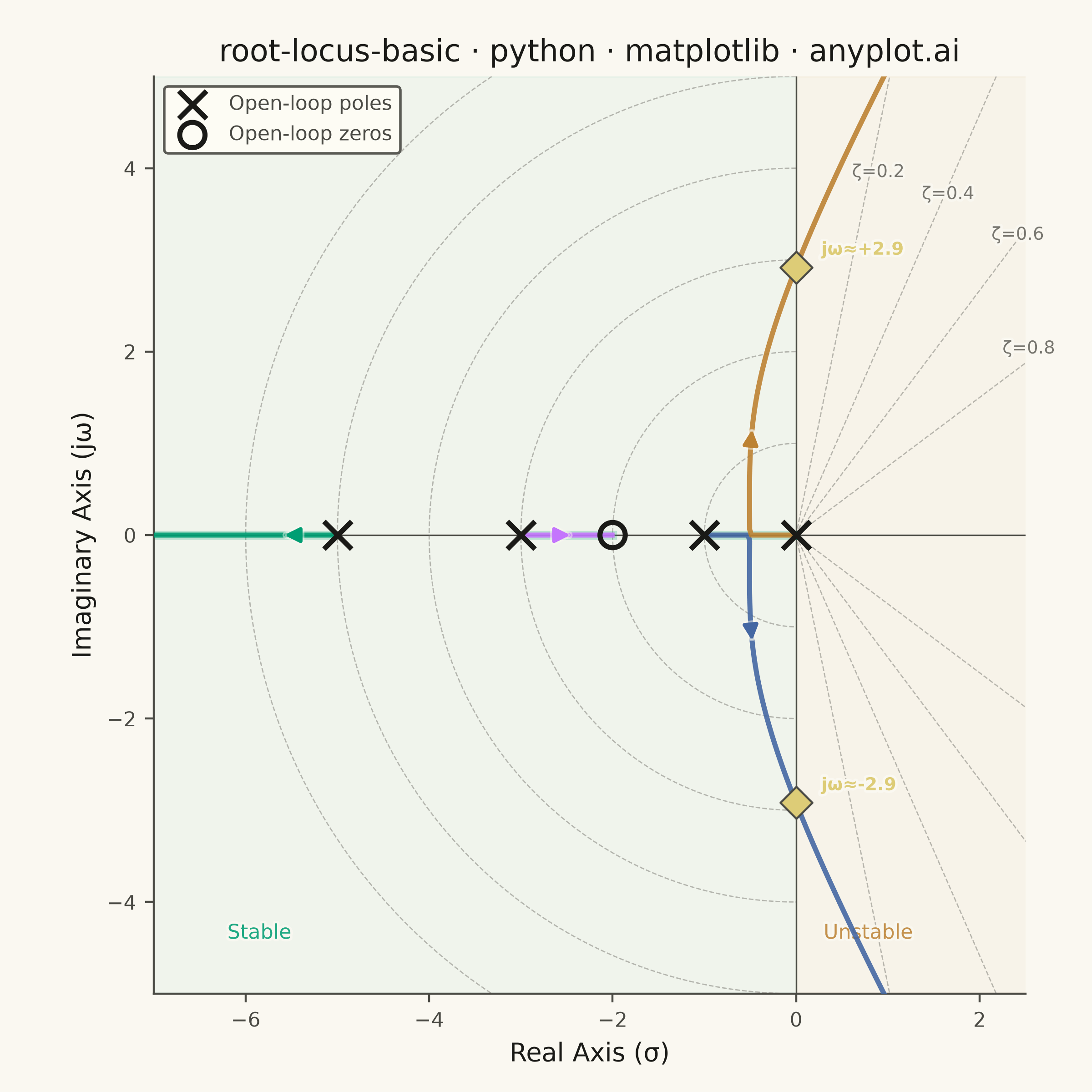
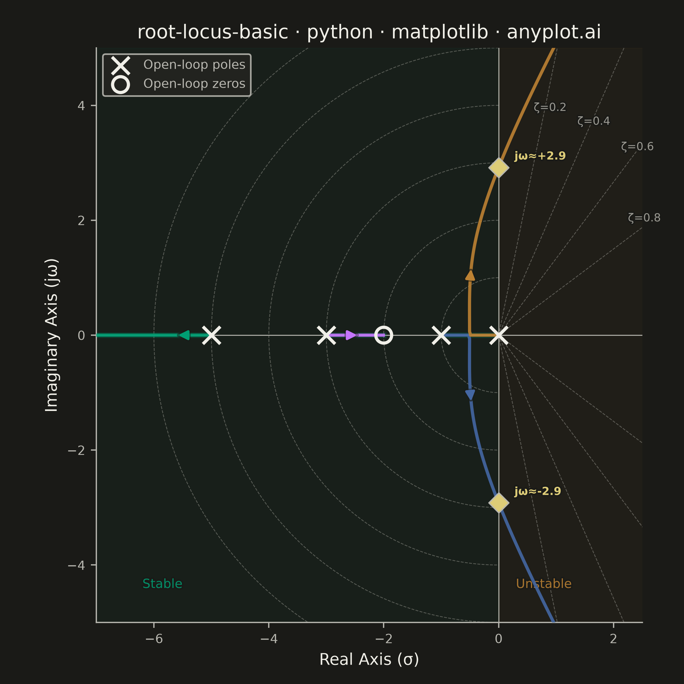
A root locus plot traces how the closed-loop poles of a transfer function migrate through the complex plane as a system parameter (typically gain K) varies from 0 to infinity. It is a fundamental tool in classical control theory for analyzing system stability and designing controllers. The plot reveals critical information about pole trajectories, stability boundaries, and gain margins.
""" anyplot.ai
root-locus-basic: Root Locus Plot for Control Systems
Library: matplotlib 3.11.0 | Python 3.13.13
Quality: 92/100 | Updated: 2026-06-17
"""

import os

import matplotlib.patches as mpatches
import matplotlib.patheffects as pe
import matplotlib.pyplot as plt
import numpy as np


# Theme
THEME = os.getenv("ANYPLOT_THEME", "light")
PAGE_BG = "#FAF8F1" if THEME == "light" else "#1A1A17"
ELEVATED_BG = "#FFFDF6" if THEME == "light" else "#242420"
INK = "#1A1A17" if THEME == "light" else "#F0EFE8"
INK_SOFT = "#4A4A44" if THEME == "light" else "#B8B7B0"
INK_MUTED = "#6B6A63" if THEME == "light" else "#A8A79F"

# Imprint palette — branches follow canonical order, first always #009E73
IMPRINT = ["#009E73", "#C475FD", "#4467A3", "#BD8233", "#AE3030", "#2ABCCD", "#954477", "#99B314"]
AMBER = "#DDCC77"  # semantic anchor: stability-boundary warning markers

# Data — G(s) = (s+2) / [s(s+1)(s+3)(s+5)], DC servo position control loop
open_loop_poles = np.array([0.0, -1.0, -3.0, -5.0])
open_loop_zeros = np.array([-2.0])

# Denominator: s(s+1)(s+3)(s+5) = s^4 + 9s^3 + 23s^2 + 15s
den_coeffs = np.array([1.0, 9.0, 23.0, 15.0, 0.0])
num_coeffs = np.array([1.0, 2.0])  # (s+2)

# Vary gain K from 0 → 1000, dense sampling near origin for smooth branches
gains = np.concatenate(
    [
        np.linspace(0, 1, 200),
        np.linspace(1, 10, 300),
        np.linspace(10, 50, 300),
        np.linspace(50, 200, 300),
        np.linspace(200, 1000, 400),
    ]
)

n_poles = len(den_coeffs) - 1
locus = np.full((len(gains), n_poles), np.nan + 1j * np.nan)

for i, K in enumerate(gains):
    num_padded = np.zeros(len(den_coeffs))
    num_padded[-len(num_coeffs) :] = num_coeffs
    char_poly = den_coeffs + K * num_padded
    roots = np.roots(char_poly)
    roots = np.sort_complex(roots)
    locus[i, :] = roots

# Sort branches by continuity (greedy nearest-neighbour tracking)
for i in range(1, len(gains)):
    prev = locus[i - 1, :]
    curr = locus[i, :].copy()
    used = np.zeros(n_poles, dtype=bool)
    order = np.zeros(n_poles, dtype=int)
    for j in range(n_poles):
        dists = np.abs(curr - prev[j])
        dists[used] = np.inf
        best = np.argmin(dists)
        order[j] = best
        used[best] = True
    locus[i, :] = curr[order]

# Find imaginary-axis crossings (stability boundary)
crossings = []
for branch in range(n_poles):
    real_parts = locus[:, branch].real
    for i in range(1, len(real_parts)):
        if real_parts[i - 1] * real_parts[i] < 0:
            t = abs(real_parts[i - 1]) / (abs(real_parts[i - 1]) + abs(real_parts[i]))
            cross_point = locus[i - 1, branch] + t * (locus[i, branch] - locus[i - 1, branch])
            crossings.append(cross_point)

# Canvas — 2400×2400 px (square: equal-aspect root locus, symmetric about real axis)
fig, ax = plt.subplots(figsize=(6, 6), dpi=400, facecolor=PAGE_BG)
ax.set_facecolor(PAGE_BG)

# Path-effect stroke uses PAGE_BG so it works in both light and dark
stroke = pe.withStroke(linewidth=2, foreground=PAGE_BG)

# Stable / unstable region shading — Imprint teal + ochre (colorblind-safe, no red/green conflict)
ax.axvspan(-10, 0, color=IMPRINT[0], alpha=0.04, zorder=0)
ax.axvspan(0, 5, color=IMPRINT[3], alpha=0.04, zorder=0)
ax.text(-6.2, -4.4, "Stable", fontsize=8, color=IMPRINT[0], alpha=0.85, path_effects=[stroke])
ax.text(0.3, -4.4, "Unstable", fontsize=8, color=IMPRINT[3], alpha=0.85, path_effects=[stroke])

# Constant damping-ratio lines (ζ = 0.2, 0.4, 0.6, 0.8)
max_r = 7
for zeta in [0.2, 0.4, 0.6, 0.8]:
    angle = np.arccos(zeta)
    r = np.linspace(0, max_r, 100)
    lx = -r * np.cos(np.pi - angle)
    ly = r * np.sin(np.pi - angle)
    ax.plot(lx, ly, "--", color=INK_MUTED, linewidth=0.5, alpha=0.45)
    ax.plot(lx, -ly, "--", color=INK_MUTED, linewidth=0.5, alpha=0.45)
    lr = 3.0 if zeta >= 0.8 else 3.8
    tx = -lr * np.cos(np.pi - angle) - 0.15
    ty = lr * np.sin(np.pi - angle) + 0.18
    ax.text(tx, ty, f"ζ={zeta}", fontsize=7, color=INK_MUTED, alpha=0.9, path_effects=[stroke])

# Constant natural-frequency arcs (ωn = 1 … 6), left half-plane only
for wn in range(1, 7):
    theta = np.linspace(np.pi / 2, 3 * np.pi / 2, 200)
    ax.plot(wn * np.cos(theta), wn * np.sin(theta), "--", color=INK_MUTED, linewidth=0.5, alpha=0.45)

# Branch colors: Imprint canonical order
branch_colors = [IMPRINT[i % len(IMPRINT)] for i in range(n_poles)]

# Draw locus branches
for branch in range(n_poles):
    ax.plot(
        locus[:, branch].real, locus[:, branch].imag, color=branch_colors[branch], linewidth=2.0, alpha=0.9, zorder=3
    )

# Directional arrows (increasing gain)
for branch in range(n_poles):
    n_pts = len(gains)
    idx = n_pts // 3
    if idx + 5 < n_pts:
        p1 = locus[idx, branch]
        p2 = locus[idx + 5, branch]
        dx, dy = p2.real - p1.real, p2.imag - p1.imag
        if np.hypot(dx, dy) > 0.005:
            ax.add_patch(
                mpatches.FancyArrowPatch(
                    (p1.real, p1.imag),
                    (p2.real, p2.imag),
                    arrowstyle="-|>",
                    color=branch_colors[branch],
                    linewidth=1.5,
                    mutation_scale=12,
                    zorder=4,
                    path_effects=[pe.withStroke(linewidth=3, foreground=PAGE_BG, alpha=0.5)],
                )
            )

# Open-loop poles (×) and zeros (○) — INK colour so they flip with theme
ax.scatter(
    open_loop_poles.real,
    np.zeros_like(open_loop_poles),
    marker="x",
    s=120,
    color=INK,
    linewidths=2.0,
    zorder=5,
    label="Open-loop poles",
)
ax.scatter(
    open_loop_zeros.real,
    np.zeros_like(open_loop_zeros),
    marker="o",
    s=100,
    facecolors="none",
    edgecolors=INK,
    linewidths=2.0,
    zorder=5,
    label="Open-loop zeros",
)

# Imaginary-axis crossings: amber diamonds (semantic: stability-boundary warning)
for cp in crossings:
    ax.scatter(cp.real, cp.imag, marker="D", s=80, color=AMBER, edgecolors=INK_SOFT, linewidths=0.8, zorder=6)
    ax.annotate(
        f"jω≈{cp.imag:+.1f}",
        xy=(cp.real, cp.imag),
        xytext=(10, 5),
        textcoords="offset points",
        fontsize=7,
        color=AMBER,
        fontweight="bold",
        path_effects=[stroke],
        zorder=7,
    )

# Real-axis segments (left of an odd count of real poles+zeros)
real_pts = np.sort(np.concatenate([open_loop_poles.real, open_loop_zeros.real]))
x_range = np.linspace(-8, 1, 5000)
on_locus = np.array([np.sum(real_pts >= x) % 2 == 1 for x in x_range])

segments = []
in_seg = False
for i, val in enumerate(on_locus):
    if val and not in_seg:
        seg_start = x_range[i]
        in_seg = True
    elif not val and in_seg:
        segments.append((seg_start, x_range[i - 1]))
        in_seg = False
if in_seg:
    segments.append((seg_start, x_range[-1]))

for s0, s1 in segments:
    ax.plot([s0, s1], [0, 0], color=IMPRINT[0], linewidth=3.5, alpha=0.22, zorder=2)

# Origin cross-hair — INK_SOFT so it adapts to theme
ax.axhline(y=0, color=INK_SOFT, linewidth=0.6, zorder=1)
ax.axvline(x=0, color=INK_SOFT, linewidth=0.6, zorder=1)

# Axis chrome — all tokens theme-adaptive
title = "root-locus-basic · python · matplotlib · anyplot.ai"
title_fontsize = max(8, round(12 * 67 / len(title))) if len(title) > 67 else 12
ax.set_title(title, fontsize=title_fontsize, fontweight="medium", color=INK)
ax.set_xlabel("Real Axis (σ)", fontsize=10, color=INK)
ax.set_ylabel("Imaginary Axis (jω)", fontsize=10, color=INK)
ax.tick_params(axis="both", labelsize=8, colors=INK_SOFT, labelcolor=INK_SOFT)
for spine in ("left", "bottom"):
    ax.spines[spine].set_color(INK_SOFT)
ax.spines["top"].set_visible(False)
ax.spines["right"].set_visible(False)

ax.set_aspect("equal")
ax.set_xlim(-7, 2.5)
ax.set_ylim(-5, 5)

# Legend
leg = ax.legend(fontsize=8, loc="upper left", framealpha=0.9)
if leg:
    leg.get_frame().set_facecolor(ELEVATED_BG)
    leg.get_frame().set_edgecolor(INK_SOFT)
    plt.setp(leg.get_texts(), color=INK_SOFT)

fig.subplots_adjust(left=0.12, right=0.96, top=0.93, bottom=0.09)
plt.savefig(f"plot-{THEME}.png", dpi=400, facecolor=PAGE_BG)
Runnable source as JSON, for any HTTP client: https://api.anyplot.ai/specs/root-locus-basic/matplotlib/code. Any spec id and library id listed in llms-full.txt fit the same URL shape; every URL below is complete and callable.
{
  "spec_id": "root-locus-basic",
  "language": "python",
  "library": "matplotlib",
  "page": "https://anyplot.ai/root-locus-basic/python/matplotlib",
  "hub": "https://anyplot.ai/root-locus-basic",
  "code_json": "https://api.anyplot.ai/specs/root-locus-basic/matplotlib/code",
  "spec_json": "https://api.anyplot.ai/specs/root-locus-basic",
  "render_light_png": "https://storage.googleapis.com/anyplot-images/plots/root-locus-basic/python/matplotlib/plot-light.png",
  "render_dark_png": "https://storage.googleapis.com/anyplot-images/plots/root-locus-basic/python/matplotlib/plot-dark.png",
  "quality_score": 92.0,
  "license": "MIT",
  "guide": "https://anyplot.ai/llms.txt"
}
Part of Root Locus Plot for Control Systems on anyplot.ai.