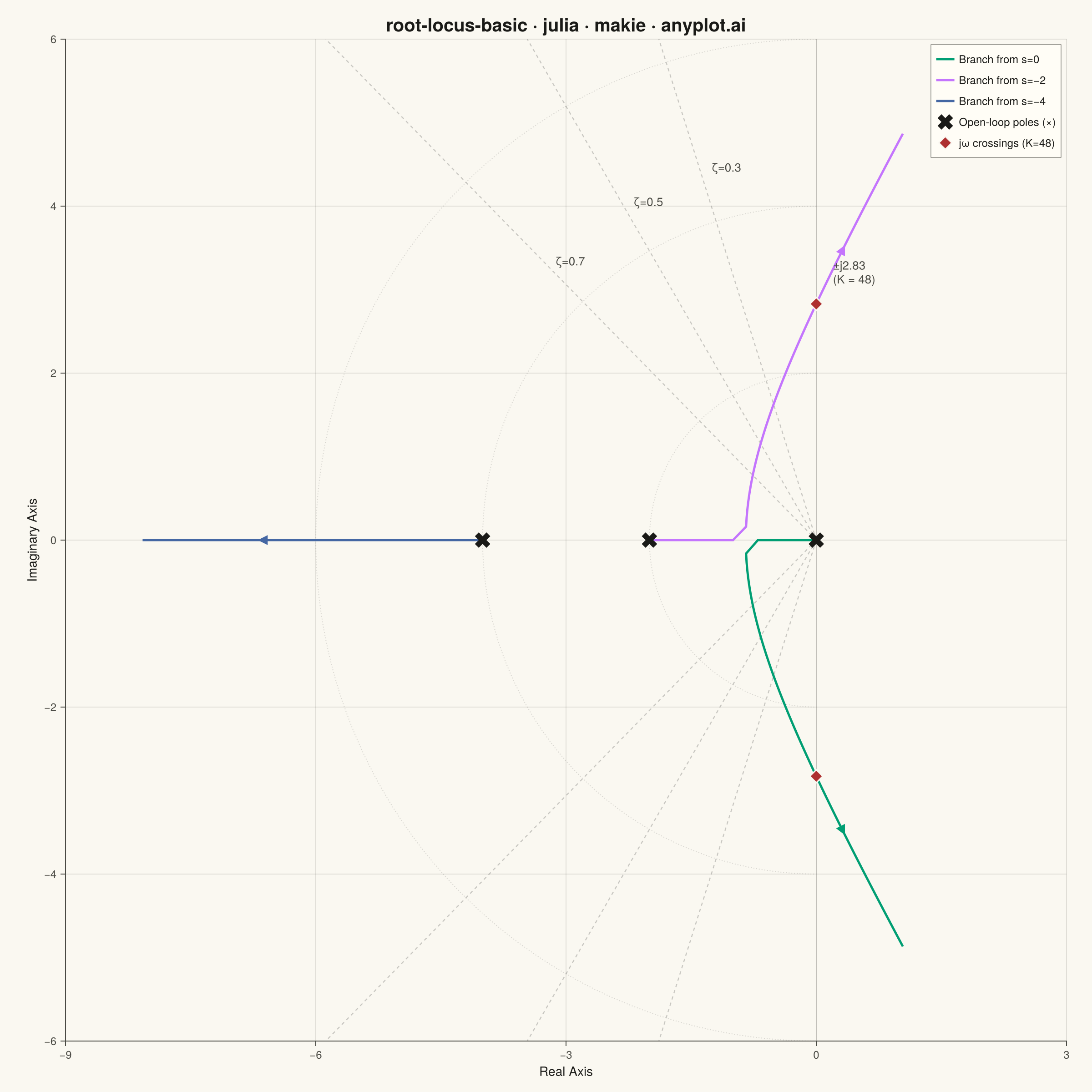
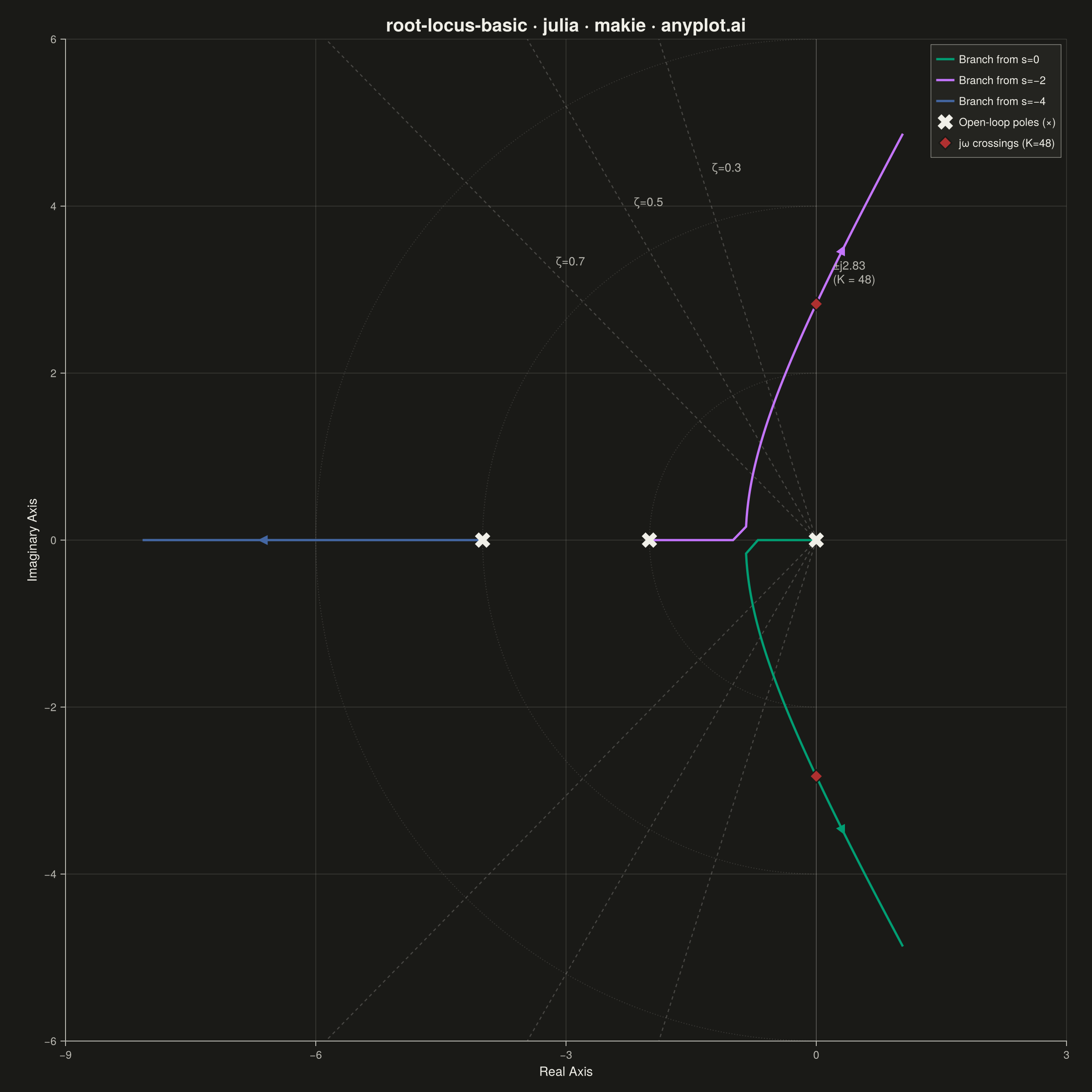
A root locus plot traces how the closed-loop poles of a transfer function migrate through the complex plane as a system parameter (typically gain K) varies from 0 to infinity. It is a fundamental tool in classical control theory for analyzing system stability and designing controllers. The plot reveals critical information about pole trajectories, stability boundaries, and gain margins.
# anyplot.ai
# root-locus-basic: Root Locus Plot for Control Systems
# Library: makie 0.22.10 | Julia 1.11.9
# Quality: 88/100 | Created: 2026-06-18

using CairoMakie
using Colors
using LinearAlgebra

# Theme tokens — Imprint palette
const THEME       = get(ENV, "ANYPLOT_THEME", "light")
const PAGE_BG     = THEME == "light" ? colorant"#FAF8F1" : colorant"#1A1A17"
const ELEVATED_BG = THEME == "light" ? colorant"#FFFDF6" : colorant"#242420"
const INK         = THEME == "light" ? colorant"#1A1A17" : colorant"#F0EFE8"
const INK_SOFT    = THEME == "light" ? colorant"#4A4A44" : colorant"#B8B7B0"
const IMPRINT     = [
    colorant"#009E73",  # 1 — brand green (first categorical series)
    colorant"#C475FD",  # 2 — lavender
    colorant"#4467A3",  # 3 — blue
    colorant"#BD8233",  # 4 — ochre
    colorant"#AE3030",  # 5 — matte red
    colorant"#2ABCCD",  # 6 — cyan
    colorant"#954477",  # 7 — rose
    colorant"#99B314",  # 8 — lime
]

# Data
# Open-loop: G(s) = K / (s(s+2)(s+4))
# Characteristic equation: s³ + 6s² + 8s + K = 0
# Open-loop poles: s = 0, −2, −4  |  No finite zeros
# Breakaway point: s ≈ −0.845 at K ≈ 3.08 (two branches merge → complex pair)
# jω-axis crossings: s = ±j√8 ≈ ±j2.83 at K = 48  (stability boundary)

const OL_POLES = [0.0, -2.0, -4.0]
const N_BR     = 3

function companion_roots(K::Float64)
    A = Float64[0   1   0
                0   0   1
               -K  -8  -6]
    return complex.(eigvals(A))  # always ComplexF64, even when roots are real
end

K_range = range(0.0002, 200.0; length = 1200)

# Sort descending by real part: branch 1 (green) ← pole at s=0 (closest to jω axis)
init = sort(companion_roots(Float64(K_range[1])), by = real, rev = true)
branches = [[c] for c in init]

for k in K_range[2:end]
    curr      = companion_roots(Float64(k))
    prev_tips = [b[end] for b in branches]
    remaining = collect(1:N_BR)
    assign    = zeros(Int, N_BR)
    for b in 1:N_BR
        best_pos, best_d = 1, Inf
        for (pos, j) in enumerate(remaining)
            d = abs(curr[j] - prev_tips[b])
            if d < best_d
                best_d   = d
                best_pos = pos
            end
        end
        assign[b] = remaining[best_pos]
        deleteat!(remaining, best_pos)
    end
    for b in 1:N_BR
        push!(branches[b], curr[assign[b]])
    end
end

bx = [real.(branches[b]) for b in 1:N_BR]
by = [imag.(branches[b]) for b in 1:N_BR]

# Grid color (INK at 12% opacity)
gc = RGBAf(INK.r, INK.g, INK.b, 0.12f0)

# Figure — square canvas → 2400×2400 output; DataAspect preserves s-plane geometry
fig = Figure(
    size            = (1200, 1200),
    fontsize        = 14,
    backgroundcolor = PAGE_BG,
)

ax = Axis(
    fig[1, 1];
    title              = "root-locus-basic · julia · makie · anyplot.ai",
    titlesize          = 20,
    titlecolor         = INK,
    xlabel             = "Real Axis",
    ylabel             = "Imaginary Axis",
    xlabelsize         = 14,
    ylabelsize         = 14,
    xlabelcolor        = INK,
    ylabelcolor        = INK,
    xticklabelsize     = 12,
    yticklabelsize     = 12,
    xticklabelcolor    = INK_SOFT,
    yticklabelcolor    = INK_SOFT,
    xtickcolor         = INK_SOFT,
    ytickcolor         = INK_SOFT,
    backgroundcolor    = PAGE_BG,
    topspinevisible    = false,
    rightspinevisible  = false,
    leftspinecolor     = INK_SOFT,
    bottomspinecolor   = INK_SOFT,
    xgridcolor         = gc,
    ygridcolor         = gc,
    xminorgridvisible  = false,
    yminorgridvisible  = false,
    aspect             = DataAspect(),
)

# Imaginary axis (stability boundary): thin vertical reference at x=0
vlines!(ax, [0.0]; color = RGBAf(INK.r, INK.g, INK.b, 0.15f0), linewidth = 1.0)

# Constant natural-frequency arcs (left half-plane semicircles, dotted)
for wn in (2.0, 4.0, 6.0)
    th = range(π / 2, 3π / 2; length = 120)
    lines!(ax, wn .* cos.(th), wn .* sin.(th);
        color     = RGBAf(INK.r, INK.g, INK.b, 0.15f0),
        linestyle = :dot,
        linewidth = 1.0,
    )
end

# Constant damping-ratio lines (dashed radial lines from origin)
for (zeta, lbl) in ((0.3, "ζ=0.3"), (0.5, "ζ=0.5"), (0.7, "ζ=0.7"))
    phi    = acos(zeta)            # angle from negative real axis
    r_ext  = 9.0
    sx, sy = -cos(phi), sin(phi)  # unit direction into upper half-plane
    col    = RGBAf(INK.r, INK.g, INK.b, 0.22f0)
    lines!(ax, [0.0, r_ext * sx], [0.0,  r_ext * sy]; color = col, linestyle = :dash, linewidth = 1.2)
    lines!(ax, [0.0, r_ext * sx], [0.0, -r_ext * sy]; color = col, linestyle = :dash, linewidth = 1.2)
    text!(ax, 0.52 * r_ext * sx + 0.15, 0.52 * r_ext * sy;
        text     = lbl,
        color    = INK_SOFT,
        fontsize = 13,
        align    = (:left, :center),
    )
end

# Locus branches with direction arrows
branch_colors = IMPRINT[1:3]
branch_labels = ["Branch from s=0", "Branch from s=−2", "Branch from s=−4"]

for b in 1:N_BR
    xs, ys = bx[b], by[b]
    lines!(ax, xs, ys; color = branch_colors[b], linewidth = 2.5, label = branch_labels[b])

    # Direction-of-increasing-K arrow (rotated triangle at 40% along branch)
    n  = length(xs)
    ai = clamp(round(Int, n * 0.40), 2, n - 1)
    dx = xs[ai + 1] - xs[ai - 1]
    dy = ys[ai + 1] - ys[ai - 1]
    scatter!(ax, [xs[ai]], [ys[ai]];
        marker      = :utriangle,
        markersize  = 15,
        color       = branch_colors[b],
        strokewidth = 0.0,
        rotation    = atan(dy, dx) - π / 2,
    )
end

# Open-loop poles (× markers)
scatter!(ax, OL_POLES, zeros(N_BR);
    marker     = :xcross,
    markersize = 24,
    color      = INK,
    label      = "Open-loop poles (×)",
)

# jω-axis crossings at K=48 (stability boundary)
jw_y = sqrt(8.0)   # ≈ 2.83
scatter!(ax, [0.0, 0.0], [jw_y, -jw_y];
    marker      = :diamond,
    markersize  = 16,
    color       = IMPRINT[5],
    strokewidth = 1.5,
    strokecolor = PAGE_BG,
    label       = "jω crossings (K=48)",
)
text!(ax, 0.2, jw_y + 0.38;
    text     = "±j$(round(jw_y; digits = 2))\n(K = 48)",
    color    = INK_SOFT,
    fontsize = 13,
    align    = (:left, :center),
)

xlims!(ax, -9.0, 3.0)
ylims!(ax, -6.0, 6.0)

axislegend(ax;
    position        = :rt,
    framecolor      = INK_SOFT,
    framewidth      = 0.5,
    backgroundcolor = ELEVATED_BG,
    labelcolor      = INK,
    labelsize       = 12,
    rowgap          = 3,
)

save(joinpath(@__DIR__, "plot-$(THEME).png"), fig; px_per_unit = 2)
Runnable source as JSON, for any HTTP client: https://api.anyplot.ai/specs/root-locus-basic/makie/code. Any spec id and library id listed in llms-full.txt fit the same URL shape; every URL below is complete and callable.
{
  "spec_id": "root-locus-basic",
  "language": "julia",
  "library": "makie",
  "page": "https://anyplot.ai/root-locus-basic/julia/makie",
  "hub": "https://anyplot.ai/root-locus-basic",
  "code_json": "https://api.anyplot.ai/specs/root-locus-basic/makie/code",
  "spec_json": "https://api.anyplot.ai/specs/root-locus-basic",
  "render_light_png": "https://storage.googleapis.com/anyplot-images/plots/root-locus-basic/julia/makie/plot-light.png",
  "render_dark_png": "https://storage.googleapis.com/anyplot-images/plots/root-locus-basic/julia/makie/plot-dark.png",
  "quality_score": 88.0,
  "license": "MIT",
  "guide": "https://anyplot.ai/llms.txt"
}
Part of Root Locus Plot for Control Systems on anyplot.ai.