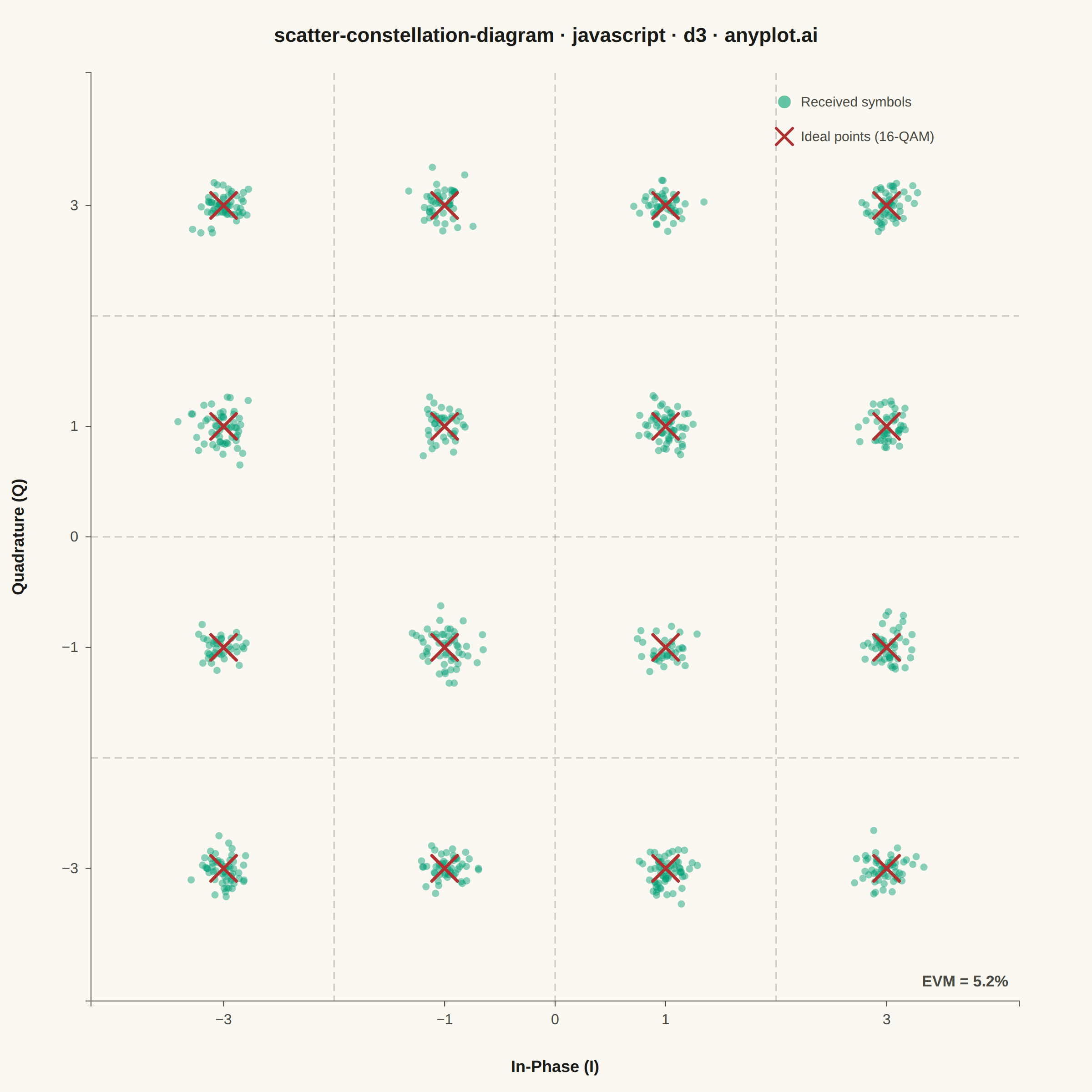
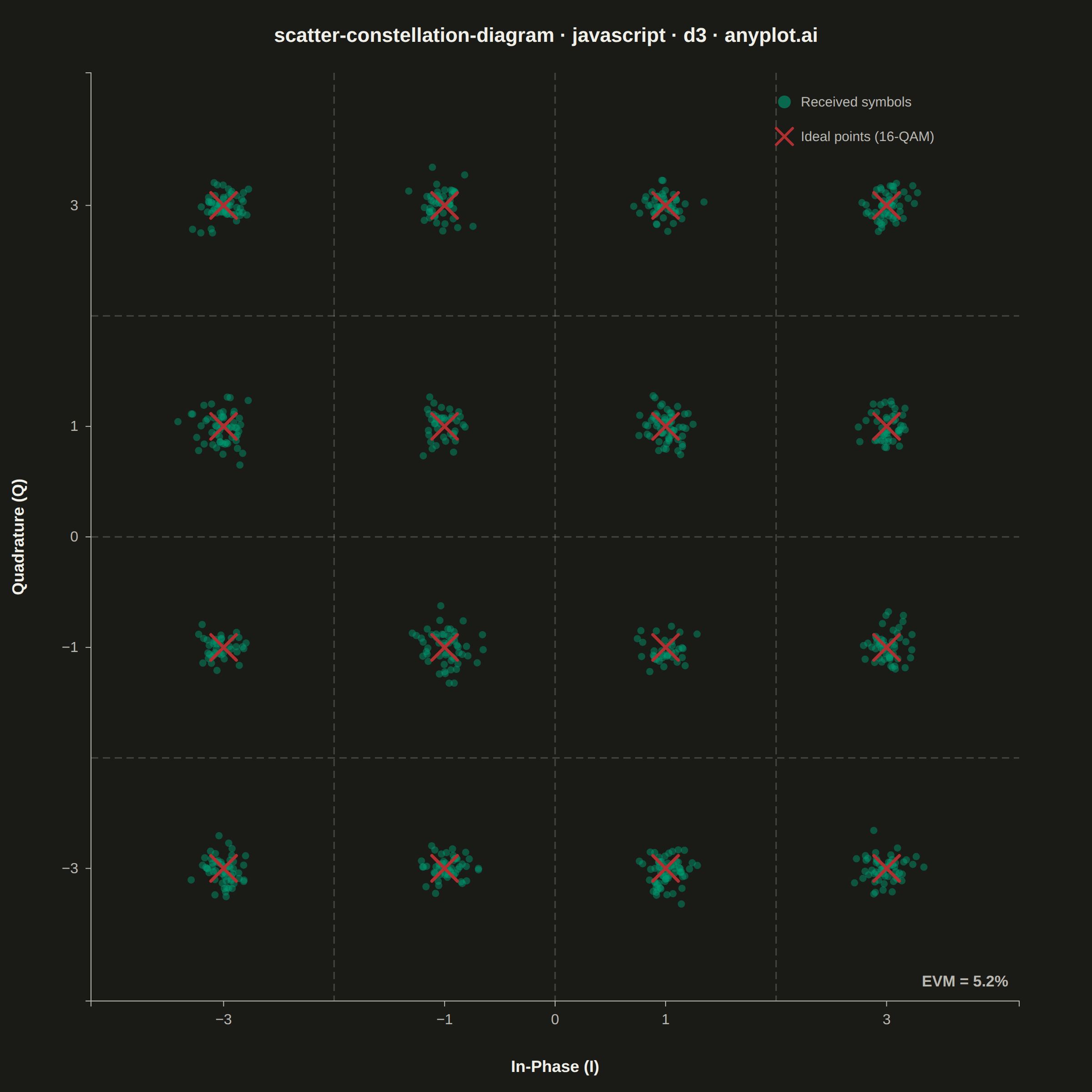
An I/Q (In-phase/Quadrature) scatter plot showing symbol positions of a digitally modulated signal. Ideal constellation points are displayed as reference markers with received symbols scattered around them, revealing modulation quality and signal impairments such as noise, phase offset, and amplitude distortion. This plot is the standard diagnostic tool for evaluating digital modulation schemes like 16-QAM.
// anyplot.ai
// scatter-constellation-diagram: Digital Modulation Constellation Diagram
// Library: d3 7.9.0 | JavaScript 22.22.3
// Quality: 90/100 | Created: 2026-06-18

//# anyplot-orientation: square

const t = window.ANYPLOT_TOKENS;
const { width, height } = window.ANYPLOT_SIZE;

// Equal margins on all sides for square inner plot (equal aspect ratio)
const margin = { top: 80, right: 80, bottom: 100, left: 100 };
const iw = width - margin.left - margin.right;
const ih = height - margin.top - margin.bottom;

// Park-Miller LCG for reproducible deterministic data (no seeded RNG in browser)
let _s = 42;
function rand() {
  _s = (_s * 16807) % 2147483647;
  return _s / 2147483647;
}
function randn() {
  return Math.sqrt(-2 * Math.log(rand())) * Math.cos(2 * Math.PI * rand());
}

// 16-QAM ideal constellation points: 4×4 grid at ±1, ±3
const levels = [-3, -1, 1, 3];
const idealPoints = [];
for (const q of levels) {
  for (const i of levels) {
    idealPoints.push({ i, q });
  }
}

// Received symbols: Gaussian noise (σ = 0.115 per dimension → EVM ≈ 5.2%)
const NOISE_STD = 0.115;
const symbols = [];
for (let k = 0; k < 800; k++) {
  const idx = Math.floor(rand() * 16);
  const ref = idealPoints[idx];
  symbols.push({ i: ref.i + randn() * NOISE_STD, q: ref.q + randn() * NOISE_STD, idx });
}

// Compute EVM from generated data
const signalPower = idealPoints.reduce((s, p) => s + p.i * p.i + p.q * p.q, 0) / idealPoints.length;
const errorPower = symbols.reduce((s, sym) => {
  const ref = idealPoints[sym.idx];
  return s + (sym.i - ref.i) ** 2 + (sym.q - ref.q) ** 2;
}, 0) / symbols.length;
const evmPct = (Math.sqrt(errorPower / signalPower) * 100).toFixed(1);

// SVG mount
const svg = d3.select("#container").append("svg")
  .attr("width", width)
  .attr("height", height);

const g = svg.append("g").attr("transform", `translate(${margin.left},${margin.top})`);

// Clip path — keeps scatter symbols inside plot bounds
svg.append("defs").append("clipPath").attr("id", "clip")
  .append("rect").attr("width", iw).attr("height", ih);

// Scales — symmetric domain, equal aspect ratio (iw === ih for square canvas)
const EXTENT = 4.2;
const x = d3.scaleLinear().domain([-EXTENT, EXTENT]).range([0, iw]);
const y = d3.scaleLinear().domain([-EXTENT, EXTENT]).range([ih, 0]);

// Decision boundary lines at 0, ±2 (midpoints between adjacent QAM symbol groups)
const boundaries = [-2, 0, 2];
const gBounds = g.append("g").attr("clip-path", "url(#clip)");

gBounds.selectAll(".bv").data(boundaries).join("line")
  .attr("x1", d => x(d)).attr("x2", d => x(d))
  .attr("y1", 0).attr("y2", ih)
  .attr("stroke", t.inkSoft)
  .attr("stroke-opacity", 0.28)
  .attr("stroke-width", 1.5)
  .attr("stroke-dasharray", "8,5");

gBounds.selectAll(".bh").data(boundaries).join("line")
  .attr("y1", d => y(d)).attr("y2", d => y(d))
  .attr("x1", 0).attr("x2", iw)
  .attr("stroke", t.inkSoft)
  .attr("stroke-opacity", 0.28)
  .attr("stroke-width", 1.5)
  .attr("stroke-dasharray", "8,5");

// Received symbols — small semi-transparent circles (Imprint palette position 1)
g.append("g").attr("clip-path", "url(#clip)")
  .selectAll("circle").data(symbols).join("circle")
  .attr("cx", d => x(d.i))
  .attr("cy", d => y(d.q))
  .attr("r", 4)
  .attr("fill", t.palette[0])
  .attr("fill-opacity", 0.45);

// Ideal constellation points — red X crosses (matte red, Imprint position 5)
const gIdeal = g.append("g");
idealPoints.forEach(pt => {
  const cx = x(pt.i);
  const cy = y(pt.q);
  const s = 14;
  gIdeal.append("line")
    .attr("x1", cx - s).attr("y1", cy - s)
    .attr("x2", cx + s).attr("y2", cy + s)
    .attr("stroke", t.palette[4])
    .attr("stroke-width", 3.5)
    .attr("stroke-linecap", "round");
  gIdeal.append("line")
    .attr("x1", cx + s).attr("y1", cy - s)
    .attr("x2", cx - s).attr("y2", cy + s)
    .attr("stroke", t.palette[4])
    .attr("stroke-width", 3.5)
    .attr("stroke-linecap", "round");
});

// Axes
const xAxisG = g.append("g")
  .attr("transform", `translate(0,${ih})`)
  .call(d3.axisBottom(x).tickValues([-3, -1, 0, 1, 3]).tickSize(6).tickPadding(8));

const yAxisG = g.append("g")
  .call(d3.axisLeft(y).tickValues([-3, -1, 0, 1, 3]).tickSize(6).tickPadding(8));

for (const ax of [xAxisG, yAxisG]) {
  ax.selectAll("text").attr("fill", t.inkSoft).style("font-size", "16px");
  ax.selectAll(".tick line").attr("stroke", t.inkSoft);
  ax.select(".domain").attr("stroke", t.inkSoft);
}

// Axis labels
svg.append("text")
  .attr("x", margin.left + iw / 2)
  .attr("y", height - 22)
  .attr("text-anchor", "middle")
  .attr("fill", t.ink)
  .style("font-size", "18px")
  .style("font-weight", "600")
  .text("In-Phase (I)");

svg.append("text")
  .attr("transform", "rotate(-90)")
  .attr("x", -(margin.top + ih / 2))
  .attr("y", 26)
  .attr("text-anchor", "middle")
  .attr("fill", t.ink)
  .style("font-size", "18px")
  .style("font-weight", "600")
  .text("Quadrature (Q)");

// EVM annotation (bottom-right of plot area)
g.append("text")
  .attr("x", iw - 12)
  .attr("y", ih - 16)
  .attr("text-anchor", "end")
  .attr("fill", t.inkSoft)
  .style("font-size", "17px")
  .style("font-weight", "700")
  .text(`EVM = ${evmPct}%`);

// Legend (upper right)
const legendItems = [
  { label: "Received symbols", color: t.palette[0], shape: "circle" },
  { label: "Ideal points (16-QAM)", color: t.palette[4], shape: "cross" },
];
const lx = iw - 270;
const ly0 = 22;
const gLeg = g.append("g");

legendItems.forEach((item, i) => {
  const ly = ly0 + i * 38;
  if (item.shape === "circle") {
    gLeg.append("circle")
      .attr("cx", lx + 12).attr("cy", ly + 10)
      .attr("r", 7)
      .attr("fill", item.color)
      .attr("fill-opacity", 0.6);
  } else {
    const s = 9;
    gLeg.append("line")
      .attr("x1", lx + 3).attr("y1", ly + 1)
      .attr("x2", lx + 21).attr("y2", ly + 19)
      .attr("stroke", item.color).attr("stroke-width", 3).attr("stroke-linecap", "round");
    gLeg.append("line")
      .attr("x1", lx + 21).attr("y1", ly + 1)
      .attr("x2", lx + 3).attr("y2", ly + 19)
      .attr("stroke", item.color).attr("stroke-width", 3).attr("stroke-linecap", "round");
  }
  gLeg.append("text")
    .attr("x", lx + 30).attr("y", ly + 15)
    .attr("fill", t.inkSoft)
    .style("font-size", "15px")
    .text(item.label);
});

// Title (60 chars — under 67 baseline, no font size scaling needed)
svg.append("text")
  .attr("x", width / 2)
  .attr("y", 46)
  .attr("text-anchor", "middle")
  .attr("fill", t.ink)
  .style("font-size", "22px")
  .style("font-weight", "600")
  .text("scatter-constellation-diagram · javascript · d3 · anyplot.ai");
Runnable source as JSON, for any HTTP client: https://api.anyplot.ai/specs/scatter-constellation-diagram/d3/code. Any spec id and library id listed in llms-full.txt fit the same URL shape; every URL below is complete and callable.
{
  "spec_id": "scatter-constellation-diagram",
  "language": "javascript",
  "library": "d3",
  "page": "https://anyplot.ai/scatter-constellation-diagram/javascript/d3",
  "hub": "https://anyplot.ai/scatter-constellation-diagram",
  "code_json": "https://api.anyplot.ai/specs/scatter-constellation-diagram/d3/code",
  "spec_json": "https://api.anyplot.ai/specs/scatter-constellation-diagram",
  "render_light_png": "https://storage.googleapis.com/anyplot-images/plots/scatter-constellation-diagram/javascript/d3/plot-light.png",
  "render_dark_png": "https://storage.googleapis.com/anyplot-images/plots/scatter-constellation-diagram/javascript/d3/plot-dark.png",
  "interactive_light_html": "https://storage.googleapis.com/anyplot-images/plots/scatter-constellation-diagram/javascript/d3/plot-light.html",
  "interactive_dark_html": "https://storage.googleapis.com/anyplot-images/plots/scatter-constellation-diagram/javascript/d3/plot-dark.html",
  "quality_score": 90.0,
  "license": "MIT",
  "guide": "https://anyplot.ai/llms.txt"
}
Part of Digital Modulation Constellation Diagram on anyplot.ai.