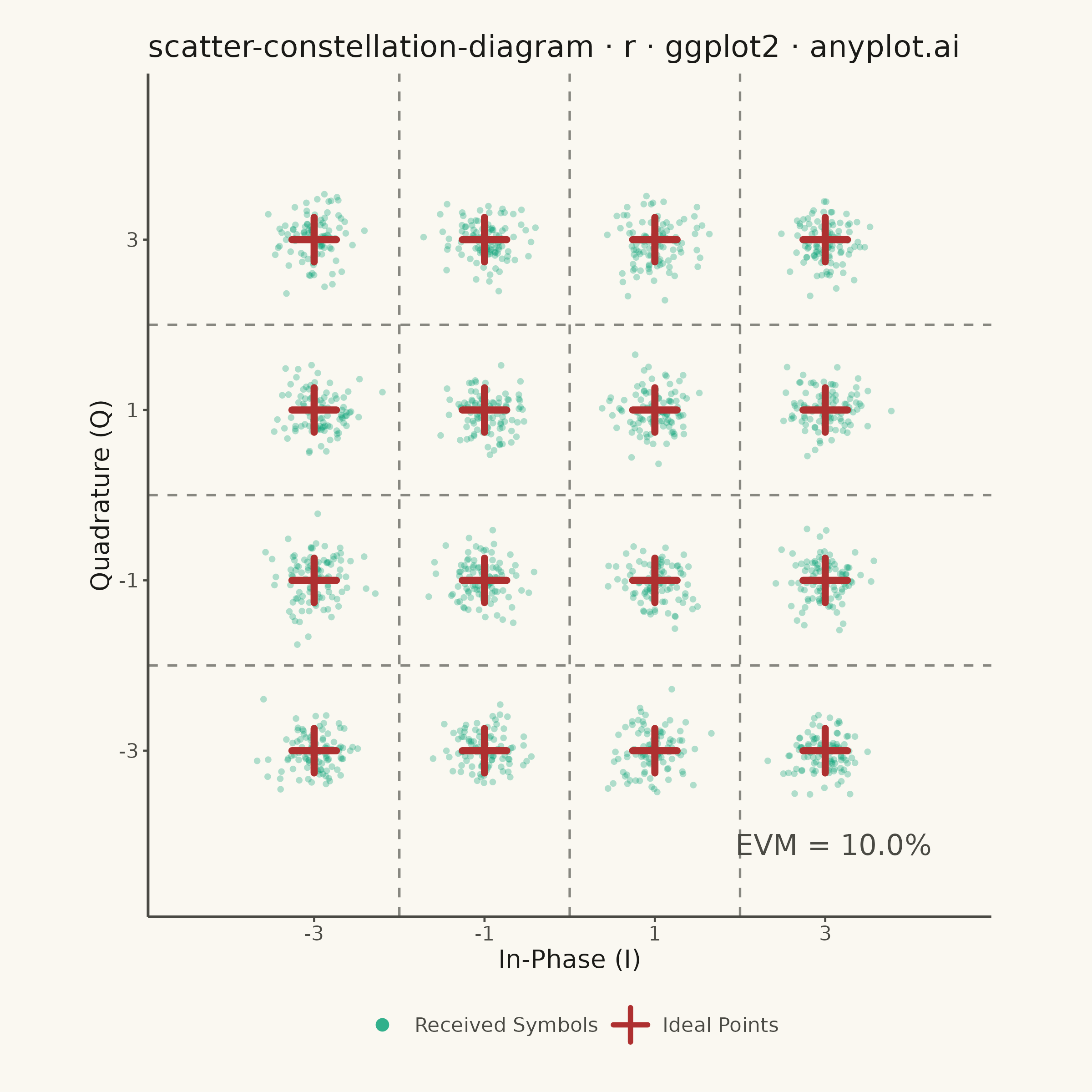
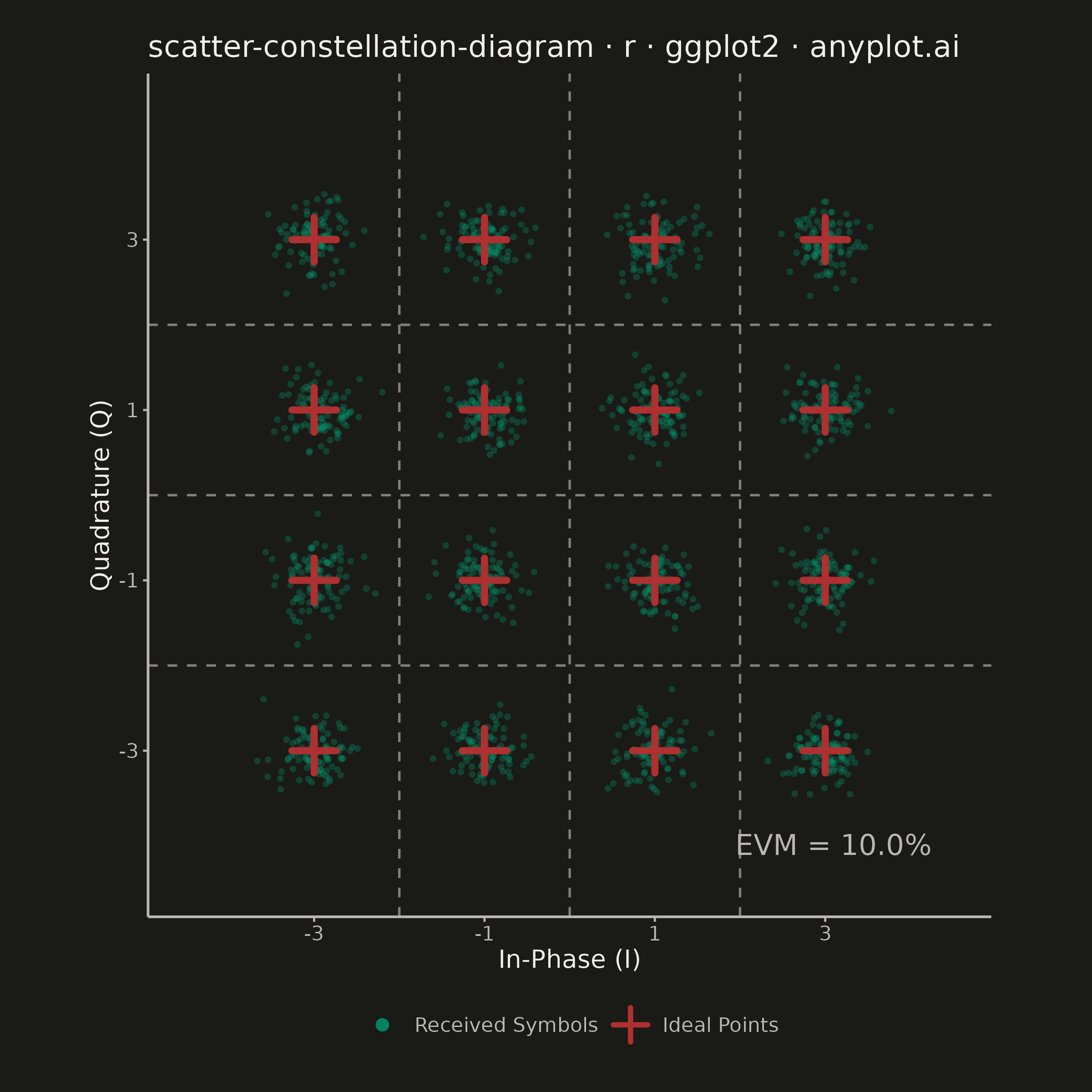
An I/Q (In-phase/Quadrature) scatter plot showing symbol positions of a digitally modulated signal. Ideal constellation points are displayed as reference markers with received symbols scattered around them, revealing modulation quality and signal impairments such as noise, phase offset, and amplitude distortion. This plot is the standard diagnostic tool for evaluating digital modulation schemes like 16-QAM.
#' anyplot.ai
#' scatter-constellation-diagram: Digital Modulation Constellation Diagram
#' Library: ggplot2 3.5.1 | R 4.4.1
#' Quality: 89/100 | Created: 2026-06-18

library(ggplot2)
library(ragg)

set.seed(42)

# --- Theme tokens ---
THEME       <- Sys.getenv("ANYPLOT_THEME", "light")
PAGE_BG     <- if (THEME == "light") "#FAF8F1" else "#1A1A17"
ELEVATED_BG <- if (THEME == "light") "#FFFDF6" else "#242420"
INK         <- if (THEME == "light") "#1A1A17" else "#F0EFE8"
INK_SOFT    <- if (THEME == "light") "#4A4A44" else "#B8B7B0"
INK_MUTED   <- if (THEME == "light") "#6B6A63" else "#A8A79F"

IMPRINT_PALETTE <- c(
  "#009E73",  # 1 brand green — received symbols
  "#C475FD",  # 2 lavender
  "#4467A3",  # 3 blue
  "#BD8233",  # 4 ochre
  "#AE3030",  # 5 matte red — ideal constellation reference points
  "#2ABCCD",  # 6 cyan
  "#954477",  # 7 rose
  "#99B314"   # 8 lime
)

# --- Data ---
# 16-QAM: 16 ideal symbol positions on a 4x4 grid at +/-1, +/-3
qam_levels <- c(-3, -1, 1, 3)
ideal_grid <- expand.grid(ideal_i = qam_levels, ideal_q = qam_levels)

# SNR ~20 dB: signal_power = mean(i^2 + q^2) = 10 across 16-QAM grid
# noise_power = signal_power / 100 = 0.1 → per-component sigma = sqrt(0.05)
n_per_point <- 100   # 1600 received symbols total
sigma       <- sqrt(0.05)

received <- do.call(rbind, lapply(seq_len(nrow(ideal_grid)), function(idx) {
  data.frame(
    i       = ideal_grid$ideal_i[idx] + rnorm(n_per_point, 0, sigma),
    q       = ideal_grid$ideal_q[idx] + rnorm(n_per_point, 0, sigma),
    ideal_i = ideal_grid$ideal_i[idx],
    ideal_q = ideal_grid$ideal_q[idx]
  )
}))

# EVM: rms error vector magnitude / rms ideal signal amplitude × 100%
error_rms  <- sqrt(mean((received$i - received$ideal_i)^2 +
                        (received$q - received$ideal_q)^2))
signal_rms <- sqrt(mean(ideal_grid$ideal_i^2 + ideal_grid$ideal_q^2))
evm_label  <- sprintf("EVM = %.1f%%", error_rms / signal_rms * 100)

# Decision boundaries fall midway between symbol rows and columns
boundaries <- c(-2, 0, 2)
axis_lim   <- c(-4.5, 4.5)

# --- Plot ---
# Title character count: ~56 < 67 baseline → default title size of 12pt
plot_title <- "scatter-constellation-diagram · r · ggplot2 · anyplot.ai"

p <- ggplot() +
  # Dashed decision-region boundaries
  geom_vline(xintercept = boundaries,
             linetype = "dashed", color = INK_SOFT, linewidth = 0.45, alpha = 0.65) +
  geom_hline(yintercept = boundaries,
             linetype = "dashed", color = INK_SOFT, linewidth = 0.45, alpha = 0.65) +
  # Received symbols — semi-transparent to reveal density clusters
  geom_point(data = received, aes(x = i, y = q, color = "Received Symbols"),
             size = 0.9, alpha = 0.30, shape = 16) +
  # Ideal constellation points — prominent cross markers (engineering convention)
  geom_point(data = ideal_grid, aes(x = ideal_i, y = ideal_q, color = "Ideal Points"),
             size = 4.5, shape = 3, stroke = 2.0) +
  # EVM annotation (bottom-right corner)
  annotate("text",
           x = 4.25, y = -4.1,
           label = evm_label,
           color = INK_SOFT, size = 4.0, hjust = 1) +
  scale_color_manual(
    values = c("Received Symbols" = IMPRINT_PALETTE[1],
               "Ideal Points"     = IMPRINT_PALETTE[5]),
    breaks = c("Received Symbols", "Ideal Points"),
    name   = NULL
  ) +
  guides(color = guide_legend(
    override.aes = list(
      shape  = c(16, 3),
      size   = c(2.5, 3.5),
      alpha  = c(0.8, 1.0),
      stroke = c(0.0, 1.5)
    )
  )) +
  scale_x_continuous(limits = axis_lim, breaks = qam_levels) +
  scale_y_continuous(limits = axis_lim, breaks = qam_levels) +
  coord_fixed() +
  labs(
    title = plot_title,
    x     = "In-Phase (I)",
    y     = "Quadrature (Q)"
  ) +
  theme_minimal(base_size = 8) +
  theme(
    plot.background   = element_rect(fill = PAGE_BG, color = PAGE_BG),
    panel.background  = element_rect(fill = PAGE_BG, color = NA),
    panel.grid.major  = element_blank(),
    panel.grid.minor  = element_blank(),
    panel.border      = element_blank(),
    axis.line         = element_line(color = INK_SOFT, linewidth = 0.5),
    axis.ticks        = element_line(color = INK_SOFT, linewidth = 0.4),
    axis.title        = element_text(color = INK, size = 10),
    axis.text         = element_text(color = INK_SOFT, size = 8),
    plot.title        = element_text(color = INK, size = 12, hjust = 0),
    plot.margin       = margin(14, 18, 14, 14, "pt"),
    legend.background = element_rect(fill = NA, color = NA),
    legend.key        = element_rect(fill = NA, color = NA),
    legend.text       = element_text(color = INK_SOFT, size = 8),
    legend.title      = element_blank(),
    legend.position   = "bottom"
  )

# --- Save ---
ggsave(
  filename = sprintf("plot-%s.png", THEME),
  plot     = p,
  device   = ragg::agg_png,
  width    = 6,
  height   = 6,
  units    = "in",
  dpi      = 400
)
Runnable source as JSON, for any HTTP client: https://api.anyplot.ai/specs/scatter-constellation-diagram/ggplot2/code. Any spec id and library id listed in llms-full.txt fit the same URL shape; every URL below is complete and callable.
{
  "spec_id": "scatter-constellation-diagram",
  "language": "r",
  "library": "ggplot2",
  "page": "https://anyplot.ai/scatter-constellation-diagram/r/ggplot2",
  "hub": "https://anyplot.ai/scatter-constellation-diagram",
  "code_json": "https://api.anyplot.ai/specs/scatter-constellation-diagram/ggplot2/code",
  "spec_json": "https://api.anyplot.ai/specs/scatter-constellation-diagram",
  "render_light_png": "https://storage.googleapis.com/anyplot-images/plots/scatter-constellation-diagram/r/ggplot2/plot-light.png",
  "render_dark_png": "https://storage.googleapis.com/anyplot-images/plots/scatter-constellation-diagram/r/ggplot2/plot-dark.png",
  "quality_score": 89.0,
  "license": "MIT",
  "guide": "https://anyplot.ai/llms.txt"
}
Part of Digital Modulation Constellation Diagram on anyplot.ai.