The same plot in 14 other libraries — JavaScript: Chart.js, D3.js, Apache ECharts, MUI X Charts; Python: Altair, Bokeh, lets-plot, Matplotlib, Plotly, plotnine, Pygal, Seaborn; R: ggplot2; Julia: Makie.jl. Compare all 15 side by side: Scatter Map with Geographic Points in Python, R, Julia and JavaScript.
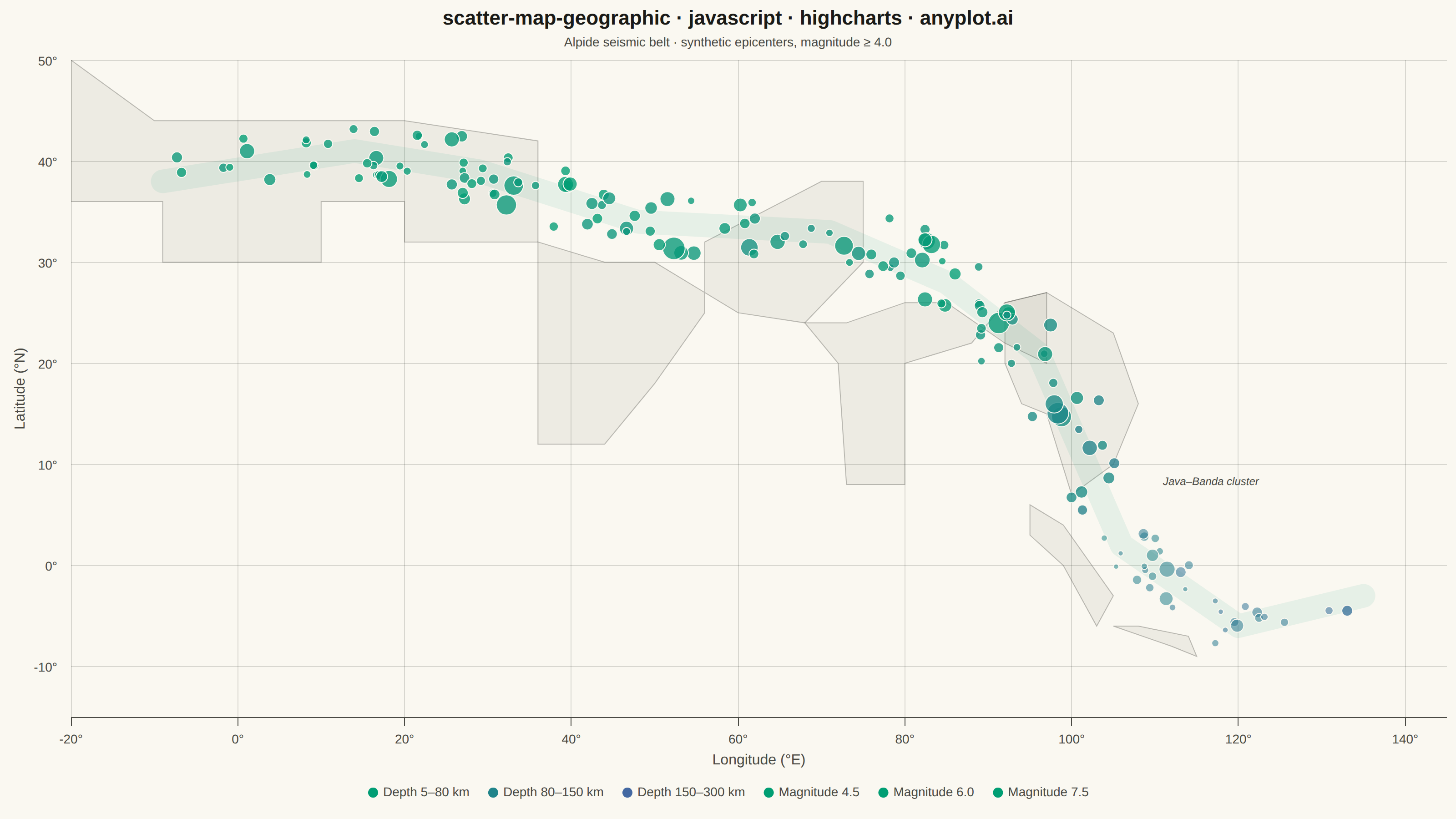
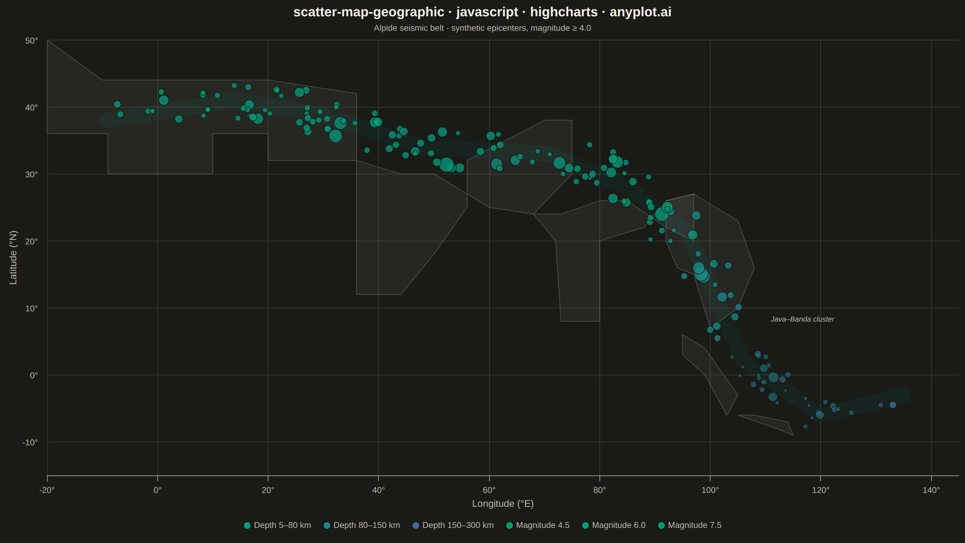
A geographic scatter plot that displays data points on a world or regional map, with each point positioned by its latitude and longitude coordinates. This visualization is ideal for showing spatial distributions of events, locations, or measurements across geographic areas. Points can optionally encode additional variables through size and color, enabling multi-dimensional geographic analysis at a glance.
// anyplot.ai
// scatter-map-geographic: Scatter Map with Geographic Points
// Library: highcharts 12.6.0 | JavaScript 22.23.2
// Quality: 93/100 | Created: 2026-09-02

//# anyplot-orientation: landscape
const t = window.ANYPLOT_TOKENS;

// --- Data (in-memory, deterministic) ----------------------------------------
// Synthetic earthquake epicenters traced along the Alpide seismic belt
// (Iberia -> Anatolia -> Himalaya -> Sunda arc). Only the core Highcharts
// bundle is loaded (no highmaps module), so geographic context comes from a
// simplified landmass outline drawn by hand with SVGRenderer (see
// "Geographic context" below) rather than a rendered map projection.
function lcg(seed) {
  let s = seed >>> 0;
  return () => {
    s = (1103515245 * s + 12345) >>> 0;
    return s / 4294967296;
  };
}
const rand = lcg(42);

const ANCHORS = [
  { lon: -9, lat: 38, depth: 20 }, // Iberia
  { lon: 14, lat: 41, depth: 15 }, // Italy
  { lon: 29, lat: 39, depth: 25 }, // Anatolia
  { lon: 48, lat: 34, depth: 35 }, // Zagros
  { lon: 71, lat: 33, depth: 70 }, // Hindu Kush
  { lon: 85, lat: 28, depth: 20 }, // Himalaya
  { lon: 96, lat: 21, depth: 90 }, // Myanmar arc
  { lon: 106, lat: 2, depth: 160 }, // Sumatra
  { lon: 120, lat: -6, depth: 210 }, // Java-Banda
  { lon: 135, lat: -3, depth: 280 }, // Banda deep
];

const MIN_MAG = 4.0;
const MAX_MAG = 7.8;
const MIN_DEPTH = 5;
const MAX_DEPTH = 300;
const POINT_COUNT = 170;

const epicenters = [];
for (let i = 0; i < POINT_COUNT; i++) {
  const along = (rand() * 0.9 + i / POINT_COUNT * 0.1 * (POINT_COUNT - 1) / POINT_COUNT) % 1;
  const span = along * (ANCHORS.length - 1);
  const idx = Math.min(Math.floor(span), ANCHORS.length - 2);
  const localT = span - idx;
  const a = ANCHORS[idx];
  const b = ANCHORS[idx + 1];

  const lonJitter = (rand() - 0.5) * 8;
  const latJitter = (rand() - 0.5) * 6;
  const depthJitter = (rand() - 0.5) * 60;

  const lon = a.lon + (b.lon - a.lon) * localT + lonJitter;
  const lat = a.lat + (b.lat - a.lat) * localT + latJitter;
  const depthBase = a.depth + (b.depth - a.depth) * localT;
  const depth = Math.min(MAX_DEPTH, Math.max(MIN_DEPTH, depthBase + depthJitter));

  // Gutenberg-Richter-like skew: many small quakes, few large ones.
  const magnitude = Math.min(MAX_MAG, MIN_MAG + -Math.log(1 - rand() * 0.98) * 0.55);

  epicenters.push({ lon, lat, magnitude, depth });
}

// --- Helpers: size + color encoding -----------------------------------------
function sizeForMagnitude(magnitude) {
  const frac = (magnitude - MIN_MAG) / (MAX_MAG - MIN_MAG);
  return 4 + frac * 16;
}

function hexToRgb(hex) {
  const n = parseInt(hex.slice(1), 16);
  return [(n >> 16) & 255, (n >> 8) & 255, n & 255];
}

function lerpColor(hexA, hexB, frac) {
  const a = hexToRgb(hexA);
  const b = hexToRgb(hexB);
  const rgb = a.map((c, i) => Math.round(c + (b[i] - c) * frac));
  return `#${rgb.map((v) => v.toString(16).padStart(2, "0")).join("")}`;
}

function colorForDepth(depth, alpha) {
  const frac = (depth - MIN_DEPTH) / (MAX_DEPTH - MIN_DEPTH);
  const hex = lerpColor(t.seq[0], t.seq[1], Math.min(1, Math.max(0, frac)));
  const [r, g, b] = hexToRgb(hex);
  return `rgba(${r}, ${g}, ${b}, ${alpha})`;
}

// The Java-Banda segment of the belt (idx 8-9 in ANCHORS) packs the most
// points into the smallest lon/lat span, so circles blur into a blob there
// even with alpha blending. Shrink + lighten markers inside that box only.
const DENSE_ZONE = { lonMin: 100, lonMax: 132, latMin: -12, latMax: 4 };
function inDenseZone(lon, lat) {
  return lon >= DENSE_ZONE.lonMin && lon <= DENSE_ZONE.lonMax && lat >= DENSE_ZONE.latMin && lat <= DENSE_ZONE.latMax;
}

// --- Chart -------------------------------------------------------------------
const epicenterSeries = {
  type: "scatter",
  name: "Epicenters",
  showInLegend: false,
  data: epicenters.map((e) => {
    const dense = inDenseZone(e.lon, e.lat);
    return {
      x: e.lon,
      y: e.lat,
      custom: { magnitude: e.magnitude, depth: e.depth },
      marker: {
        radius: sizeForMagnitude(e.magnitude) * (dense ? 0.7 : 1),
        fillColor: colorForDepth(e.depth, dense ? 0.55 : 0.78),
        lineColor: t.pageBg,
        lineWidth: 1,
      },
    };
  }),
};

// Dummy legend-only series — a standard Highcharts technique for a manual
// legend (no interactive module is required; the swatches use the exact same
// colorForDepth / sizeForMagnitude formulas the real points use).
// Representative depths pushed toward each bin's extreme (rather than its
// midpoint) so the three swatches span a wider slice of the imprint_seq
// gradient and stay visually distinguishable at a glance.
const depthLegend = [
  { label: "Depth 5–80 km", depth: 10 },
  { label: "Depth 80–150 km", depth: 145 },
  { label: "Depth 150–300 km", depth: 295 },
].map((bin) => ({
  type: "scatter",
  name: bin.label,
  showInLegend: true,
  enableMouseTracking: false,
  data: [],
  marker: { radius: 9, fillColor: colorForDepth(bin.depth, 1), lineColor: t.pageBg, lineWidth: 1 },
}));

const magnitudeLegend = [
  { label: "Magnitude 4.5", magnitude: 4.5 },
  { label: "Magnitude 6.0", magnitude: 6.0 },
  { label: "Magnitude 7.5", magnitude: 7.5 },
].map((bin) => ({
  type: "scatter",
  name: bin.label,
  showInLegend: true,
  enableMouseTracking: false,
  data: [],
  marker: { radius: sizeForMagnitude(bin.magnitude), fillColor: t.palette[0], lineColor: t.pageBg, lineWidth: 1 },
}));

// --- Geographic context (SVGRenderer, since highmaps is off-limits) ---------
// Simplified landmass silhouettes (lon/lat polygons, deliberately coarse —
// this is visual orientation, not a surveyed coastline) for the regions the
// belt crosses: S. Europe/N. Africa, Middle East, India, mainland SE Asia,
// Sumatra, Java. Drawn on chart.events.render via renderer.path() + toPixels()
// so it re-projects with the axes — a Highcharts-native technique with no
// direct equivalent in a generic <canvas>-based chart library.
const LANDMASSES = [
  [[-20, 50], [-20, 36], [-9, 36], [-9, 30], [10, 30], [10, 36], [20, 36], [20, 32], [36, 32], [36, 42], [20, 44], [0, 44], [-10, 44], [-20, 50]],
  [[36, 32], [36, 12], [44, 12], [50, 18], [56, 25], [56, 32], [70, 38], [75, 38], [75, 30], [68, 24], [60, 25], [50, 30], [44, 30], [36, 32]],
  [[68, 24], [72, 20], [73, 8], [80, 8], [80, 20], [88, 22], [92, 26], [97, 27], [97, 20], [92, 22], [85, 26], [80, 26], [73, 24], [68, 24]],
  [[92, 26], [97, 27], [105, 23], [108, 16], [105, 10], [100, 7], [97, 15], [94, 16], [92, 20], [92, 26]],
  [[95, 6], [99, 4], [105, -3], [103, -6], [99, 0], [95, 3], [95, 6]],
  [[105, -6], [112, -8], [115, -9], [114, -7], [108, -6], [105, -6]],
];

function drawGeoContext(chart) {
  if (chart.customGeo) {
    chart.customGeo.forEach((el) => el.destroy());
  }
  chart.customGeo = [];

  const xAxis = chart.xAxis[0];
  const yAxis = chart.yAxis[0];
  if (!chart.customClip) {
    chart.customClip = chart.renderer.clipRect(chart.plotLeft, chart.plotTop, chart.plotWidth, chart.plotHeight);
  } else {
    chart.customClip.attr({ x: chart.plotLeft, y: chart.plotTop, width: chart.plotWidth, height: chart.plotHeight });
  }

  const toPath = (points) =>
    points.map((pt, i) => (i === 0 ? ["M", xAxis.toPixels(pt[0]), yAxis.toPixels(pt[1])] : ["L", xAxis.toPixels(pt[0]), yAxis.toPixels(pt[1])])).concat([["Z"]]);

  LANDMASSES.forEach((poly) => {
    chart.customGeo.push(
      chart.renderer
        .path(toPath(poly))
        .attr({ fill: t.grid, "fill-opacity": 0.4, stroke: t.inkSoft, "stroke-width": 1, "stroke-opacity": 0.35, zIndex: 1 })
        .clip(chart.customClip)
        .add()
    );
  });

  // Soft translucent ribbon tracing the seismic-belt corridor itself.
  const beltPath = ANCHORS.map((a, i) => (i === 0 ? ["M", xAxis.toPixels(a.lon), yAxis.toPixels(a.lat)] : ["L", xAxis.toPixels(a.lon), yAxis.toPixels(a.lat)]));
  chart.customGeo.push(
    chart.renderer
      .path(beltPath)
      .attr({ stroke: t.palette[0], "stroke-width": 26, "stroke-opacity": 0.08, "stroke-linecap": "round", "stroke-linejoin": "round", fill: "none", zIndex: 2 })
      .clip(chart.customClip)
      .add()
  );

  // Callout labeling the densest cluster (Java-Banda) for orientation,
  // anchored above the cluster in open space so it clears both the markers
  // and the trailing Banda-deep point further along the belt.
  const calloutX = xAxis.toPixels(112) - 10;
  const calloutY = yAxis.toPixels(8);
  chart.customGeo.push(
    chart.renderer
      .text("Java–Banda cluster", calloutX, calloutY)
      .css({ color: t.inkSoft, fontSize: "12px", fontStyle: "italic" })
      .attr({ zIndex: 5 })
      .add()
  );
}

Highcharts.chart("container", {
  chart: {
    type: "scatter",
    backgroundColor: "transparent",
    animation: false,
    style: { fontFamily: "inherit" },
    zooming: { type: "xy" }, // drag-select zoom + pan for exploring point clusters (core feature)
    events: { render: function () { drawGeoContext(this); } },
  },
  credits: { enabled: false },
  colors: t.palette,
  title: {
    text: "scatter-map-geographic · javascript · highcharts · anyplot.ai",
    style: { color: t.ink, fontSize: "22px", fontWeight: "600" },
  },
  subtitle: {
    text: "Alpide seismic belt · synthetic epicenters, magnitude ≥ 4.0",
    style: { color: t.inkSoft, fontSize: "14px" },
  },
  xAxis: {
    min: -20,
    max: 145,
    tickInterval: 20,
    title: { text: "Longitude (°E)", style: { color: t.inkSoft, fontSize: "16px" } },
    lineColor: t.inkSoft,
    tickColor: t.inkSoft,
    gridLineColor: t.grid,
    gridLineWidth: 1,
    labels: { style: { color: t.inkSoft, fontSize: "14px" }, format: "{value}°" },
  },
  yAxis: {
    min: -15,
    max: 50,
    tickInterval: 10,
    startOnTick: false,
    endOnTick: false,
    title: { text: "Latitude (°N)", style: { color: t.inkSoft, fontSize: "16px" } },
    lineColor: t.inkSoft,
    tickColor: t.inkSoft,
    gridLineColor: t.grid,
    gridLineWidth: 1,
    labels: { style: { color: t.inkSoft, fontSize: "14px" }, format: "{value}°" },
  },
  legend: {
    itemStyle: { color: t.inkSoft, fontSize: "14px" },
    itemHoverStyle: { color: t.ink },
    symbolHeight: 12,
    symbolWidth: 12,
    symbolRadius: 6,
  },
  tooltip: {
    backgroundColor: t.elevatedBg,
    borderColor: t.inkSoft,
    style: { color: t.ink, fontSize: "14px" },
    pointFormatter: function () {
      return (
        `Lon ${this.x.toFixed(1)}°, Lat ${this.y.toFixed(1)}°<br/>` +
        `Magnitude ${this.custom.magnitude.toFixed(1)}<br/>` +
        `Depth ${Math.round(this.custom.depth)} km`
      );
    },
  },
  plotOptions: {
    series: { animation: false },
    scatter: { marker: { symbol: "circle" } },
  },
  series: [epicenterSeries, ...depthLegend, ...magnitudeLegend],
});
Runnable source as JSON, for any HTTP client: https://api.anyplot.ai/specs/scatter-map-geographic/highcharts/code. Any spec id and library id listed in llms-full.txt fit the same URL shape; every URL below is complete and callable.
{
  "spec_id": "scatter-map-geographic",
  "language": "javascript",
  "library": "highcharts",
  "page": "https://anyplot.ai/scatter-map-geographic/javascript/highcharts",
  "hub": "https://anyplot.ai/scatter-map-geographic",
  "code_json": "https://api.anyplot.ai/specs/scatter-map-geographic/highcharts/code",
  "spec_json": "https://api.anyplot.ai/specs/scatter-map-geographic",
  "render_light_png": "https://storage.googleapis.com/anyplot-images/plots/scatter-map-geographic/javascript/highcharts/plot-light.png",
  "render_dark_png": "https://storage.googleapis.com/anyplot-images/plots/scatter-map-geographic/javascript/highcharts/plot-dark.png",
  "interactive_light_html": "https://storage.googleapis.com/anyplot-images/plots/scatter-map-geographic/javascript/highcharts/plot-light.html",
  "interactive_dark_html": "https://storage.googleapis.com/anyplot-images/plots/scatter-map-geographic/javascript/highcharts/plot-dark.html",
  "quality_score": 93.0,
  "license": "MIT",
  "guide": "https://anyplot.ai/llms.txt"
}
Part of Scatter Map with Geographic Points on anyplot.ai.