The same plot in 14 other libraries — Python: Altair, Bokeh, lets-plot, Matplotlib, Plotly, plotnine, Pygal, Seaborn; R: ggplot2; JavaScript: Chart.js, D3.js, Apache ECharts, Highcharts, MUI X Charts. Compare all 15 side by side: Scatter Map with Geographic Points in Python, R, Julia and JavaScript.
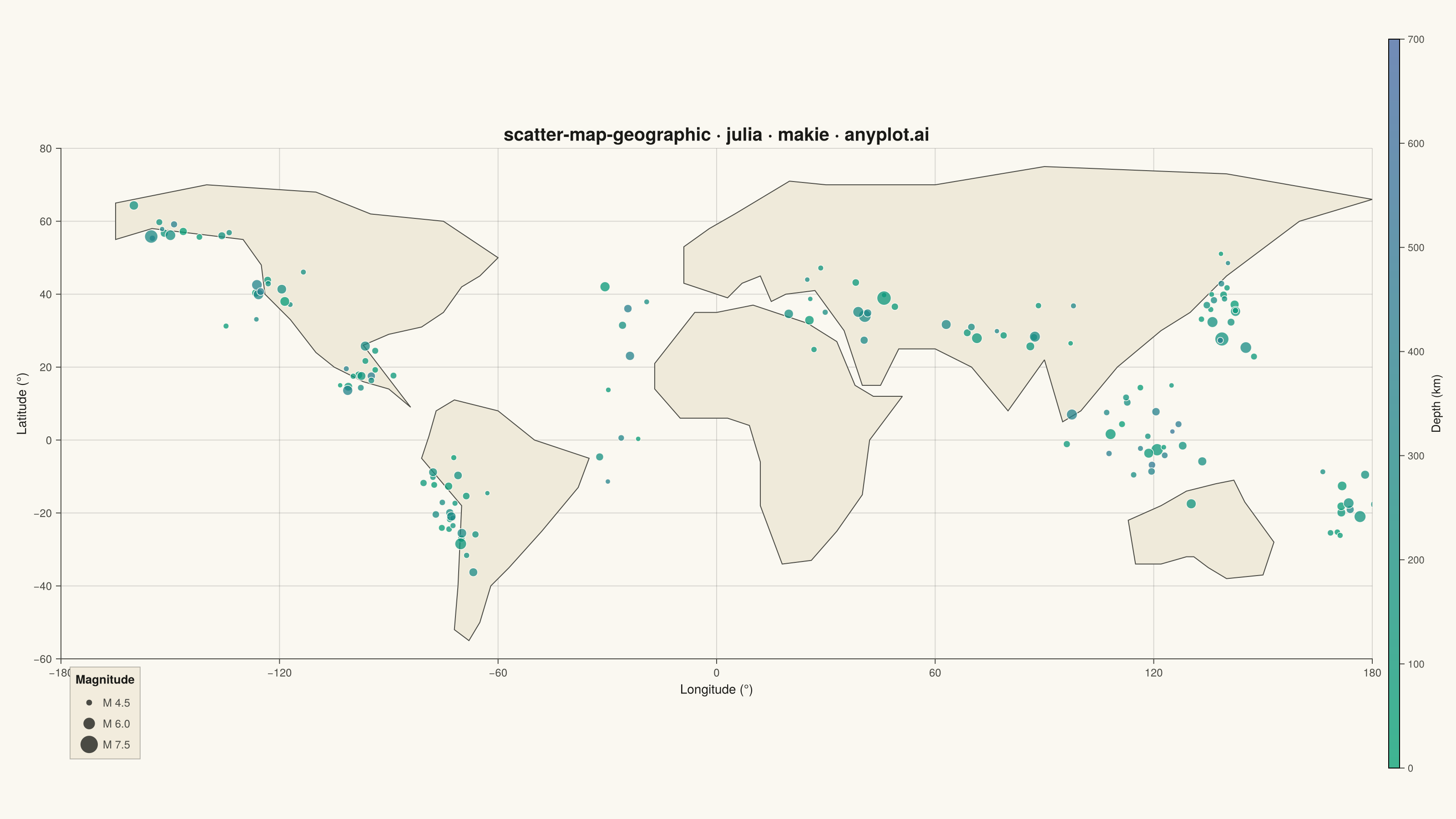
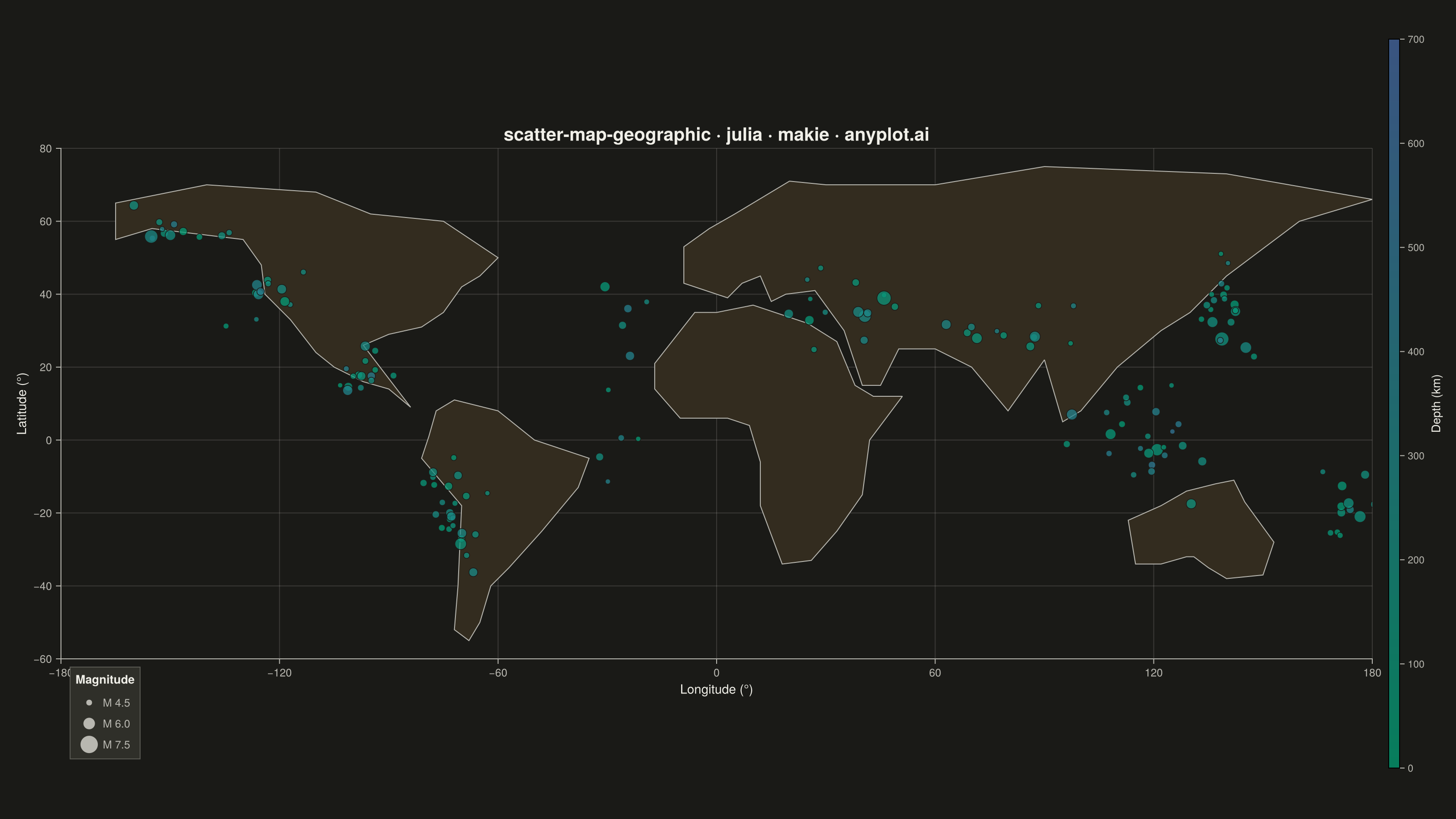
A geographic scatter plot that displays data points on a world or regional map, with each point positioned by its latitude and longitude coordinates. This visualization is ideal for showing spatial distributions of events, locations, or measurements across geographic areas. Points can optionally encode additional variables through size and color, enabling multi-dimensional geographic analysis at a glance.
# anyplot.ai
# scatter-map-geographic: Scatter Map with Geographic Points
# Library: makie 0.21.9 | Julia 1.11.9
# Quality: 91/100 | Created: 2026-09-02

using CairoMakie
using Colors
using Random

Random.seed!(42)

# --- Theme tokens -------------------------------------------------------
THEME       = get(ENV, "ANYPLOT_THEME", "light")
PAGE_BG     = THEME == "light" ? colorant"#FAF8F1" : colorant"#1A1A17"
ELEVATED_BG = THEME == "light" ? colorant"#F2ECDD" : colorant"#2F2F29"
INK         = THEME == "light" ? colorant"#1A1A17" : colorant"#F0EFE8"
INK_SOFT    = THEME == "light" ? colorant"#4A4A44" : colorant"#B8B7B0"
LAND_FILL   = THEME == "light" ? colorant"#EFEADA" : colorant"#332C1F"

IMPRINT_SEQ = cgrad([colorant"#009E73", colorant"#4467A3"])

# --- Basemap: simplified continent silhouettes (equirectangular) -------
# CairoMakie has no bundled world-map dataset (GeoMakie / NaturalEarth are
# not installed), so the coastlines below are hand-digitized low-resolution
# outlines — enough vertices to read as continents, not a survey product.
north_america = Point2f.(
    [-165, -165, -155, -130, -125, -124, -117, -110, -105, -97, -90, -84,
     -97, -90, -81, -75, -70, -65, -60, -75, -95, -110, -140, -165],
    [65, 55, 58, 55, 48, 40, 33, 24, 20, 16, 14, 9,
     26, 29, 31, 35, 42, 45, 50, 60, 62, 68, 70, 65],
)
south_america = Point2f.(
    [-77, -72, -60, -50, -35, -38, -48, -57, -62, -65, -68, -72, -71, -70,
     -81, -79, -77],
    [8, 11, 8, 0, -5, -13, -25, -35, -40, -50, -55, -52, -40, -18,
     -5, 1, 8],
)
africa = Point2f.(
    [-17, -17, -10, 3, 9, 12, 12, 18, 26, 33, 40, 42, 51, 43, 38, 33, 25,
     10, 0, -6, -17],
    [21, 14, 6, 6, 4, -6, -18, -34, -33, -25, -15, 0, 12, 12, 15, 27, 32,
     37, 35, 35, 21],
)
# Europe and Asia are one contiguous landmass at this simplification level —
# a single Eurasia ring avoids a spurious seam where two separate rings
# would otherwise leave a gap near the Urals.
eurasia = Point2f.(
    [-9, -9, -2, 5, 20, 30, 60, 90, 140, 180, 160, 140, 130, 122, 110, 100,
     95, 90, 80, 70, 60, 50, 45, 40, 35, 27, 19, 15, 12, 7, 3, -9],
    [43, 53, 58, 62, 71, 70, 70, 75, 73, 66, 60, 45, 35, 30, 20, 8,
     5, 22, 8, 20, 25, 25, 15, 15, 30, 41, 40, 38, 45, 43, 39, 43],
)
australia = Point2f.(
    [113, 122, 129, 137, 142, 145, 153, 150, 140, 135, 131, 129, 122, 115, 113],
    [-22, -18, -14, -12, -11, -17, -28, -37, -38, -35, -32, -32, -34, -34, -22],
)
continents = (north_america, south_america, africa, eurasia, australia)

# --- Data: global earthquake epicenters (magnitude + depth) ------------
# Loosely follows real seismic belts (Ring of Fire, Alpide belt, mid-ocean
# ridges) so the spatial pattern reads as plausible rather than uniform noise.
clusters = [
    (-72, -20, 4, 8, 25),    # Peru-Chile subduction zone
    (-100, 17, 5, 5, 15),    # Mexico / Central America
    (-122, 38, 4, 6, 12),    # California / Pacific Northwest
    (-155, 57, 8, 3, 12),    # Alaska / Aleutians
    (140, 37, 4, 5, 20),     # Japan
    (118, -3, 8, 8, 25),     # Indonesia / Philippines
    (175, -20, 6, 10, 15),   # Tonga / New Zealand
    (35, 37, 10, 5, 15),     # Mediterranean / Anatolia
    (85, 30, 10, 4, 12),     # Himalayan front
    (-25, 5, 5, 30, 10),     # Mid-Atlantic ridge
]

longitude = Float64[]
latitude  = Float64[]
for (clon, clat, lon_spread, lat_spread, n) in clusters
    append!(longitude, clon .+ randn(n) .* lon_spread)
    append!(latitude, clat .+ randn(n) .* lat_spread)
end
latitude = clamp.(latitude, -70, 78)

n_points  = length(longitude)
magnitude = clamp.(4.3 .+ abs.(randn(n_points)) .* 0.9, 4.0, 8.3)
depth_km  = clamp.(30 .+ abs.(randn(n_points)) .* 180, 5, 700)

mag_to_size(m) = 6 + (m - 4.0) * 6.0

# --- Plot ----------------------------------------------------------------
fig = Figure(
    resolution      = (1600, 900),
    fontsize        = 14,
    backgroundcolor = PAGE_BG,
)

ax = Axis(
    fig[1, 1];
    title              = "scatter-map-geographic · julia · makie · anyplot.ai",
    titlesize          = 20,
    titlecolor         = INK,
    xlabel             = "Longitude (°)",
    ylabel             = "Latitude (°)",
    xlabelsize         = 14,
    ylabelsize         = 14,
    xlabelcolor        = INK,
    ylabelcolor        = INK,
    xticklabelsize     = 12,
    yticklabelsize     = 12,
    xticklabelcolor    = INK_SOFT,
    yticklabelcolor    = INK_SOFT,
    xtickcolor         = INK_SOFT,
    ytickcolor         = INK_SOFT,
    xticks             = -180:60:180,
    yticks             = -60:20:80,
    backgroundcolor    = PAGE_BG,
    topspinevisible    = false,
    rightspinevisible  = false,
    leftspinecolor     = INK_SOFT,
    bottomspinecolor   = INK_SOFT,
    xgridcolor         = RGBAf(INK.r, INK.g, INK.b, 0.15),
    ygridcolor         = RGBAf(INK.r, INK.g, INK.b, 0.15),
    xminorgridvisible  = false,
    yminorgridvisible  = false,
    # Plate-carree/equirectangular (raw lon/lat with DataAspect()), not a true
    # Natural-Earth/Robinson projection — CairoMakie has no GeoMakie projection
    # support installed, so this is an intentional, documented simplification.
    aspect             = DataAspect(),
)
xlims!(ax, -180, 180)
ylims!(ax, -60, 80)

for outline in continents
    poly!(ax, outline; color = LAND_FILL, strokecolor = INK_SOFT, strokewidth = 1)
end

sc = scatter!(
    ax, longitude, latitude;
    markersize  = mag_to_size.(magnitude),
    color       = depth_km,
    colormap    = IMPRINT_SEQ,
    colorrange  = (0, 700),
    alpha       = 0.75,
    strokewidth = 0.75,
    strokecolor = PAGE_BG,
)

Colorbar(
    fig[1, 2], sc;
    label          = "Depth (km)",
    labelcolor     = INK,
    labelsize      = 13,
    ticklabelsize  = 11,
    ticklabelcolor = INK_SOFT,
    tickcolor      = INK_SOFT,
)

legend_magnitudes = [4.5, 6.0, 7.5]
legend_elements = [
    MarkerElement(marker = :circle, color = INK_SOFT, markersize = mag_to_size(m))
    for m in legend_magnitudes
]
Legend(
    fig[1, 1], legend_elements, ["M $(m)" for m in legend_magnitudes], "Magnitude";
    tellwidth       = false,
    tellheight      = false,
    halign          = :left,
    valign          = :bottom,
    margin          = (10, 10, 10, 10),
    backgroundcolor = ELEVATED_BG,
    framevisible    = true,
    framecolor      = RGBAf(INK_SOFT.r, INK_SOFT.g, INK_SOFT.b, 0.35),
    framewidth      = 1,
    labelcolor      = INK_SOFT,
    titlecolor      = INK,
    labelsize       = 12,
    titlesize       = 13,
    patchsize       = (20, 20),
)

# --- Save ------------------------------------------------------------------
save("plot-$(THEME).png", fig; px_per_unit = 2)
Runnable source as JSON, for any HTTP client: https://api.anyplot.ai/specs/scatter-map-geographic/makie/code. Any spec id and library id listed in llms-full.txt fit the same URL shape; every URL below is complete and callable.
{
  "spec_id": "scatter-map-geographic",
  "language": "julia",
  "library": "makie",
  "page": "https://anyplot.ai/scatter-map-geographic/julia/makie",
  "hub": "https://anyplot.ai/scatter-map-geographic",
  "code_json": "https://api.anyplot.ai/specs/scatter-map-geographic/makie/code",
  "spec_json": "https://api.anyplot.ai/specs/scatter-map-geographic",
  "render_light_png": "https://storage.googleapis.com/anyplot-images/plots/scatter-map-geographic/julia/makie/plot-light.png",
  "render_dark_png": "https://storage.googleapis.com/anyplot-images/plots/scatter-map-geographic/julia/makie/plot-dark.png",
  "quality_score": 91.0,
  "license": "MIT",
  "guide": "https://anyplot.ai/llms.txt"
}
Part of Scatter Map with Geographic Points on anyplot.ai.