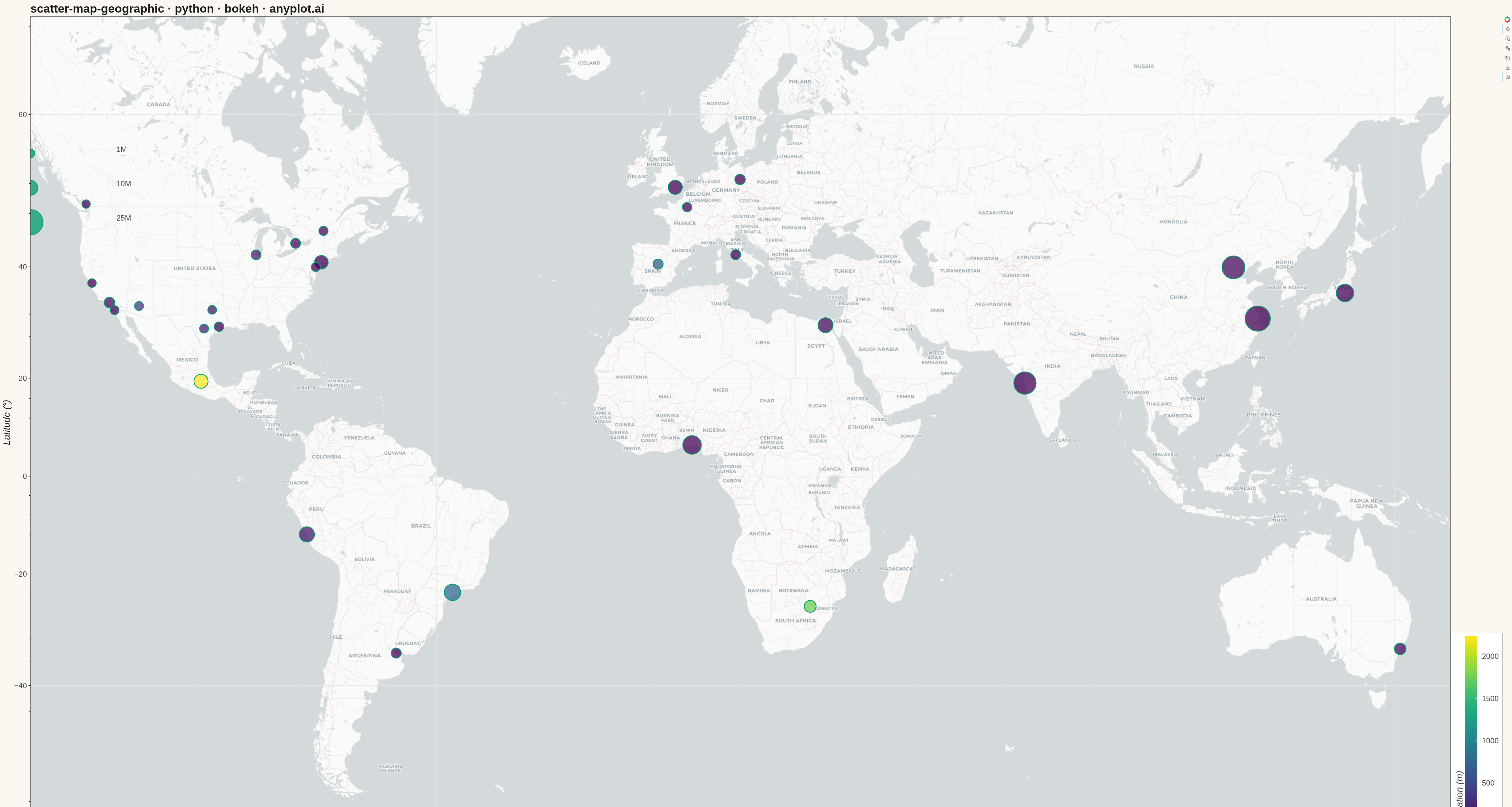
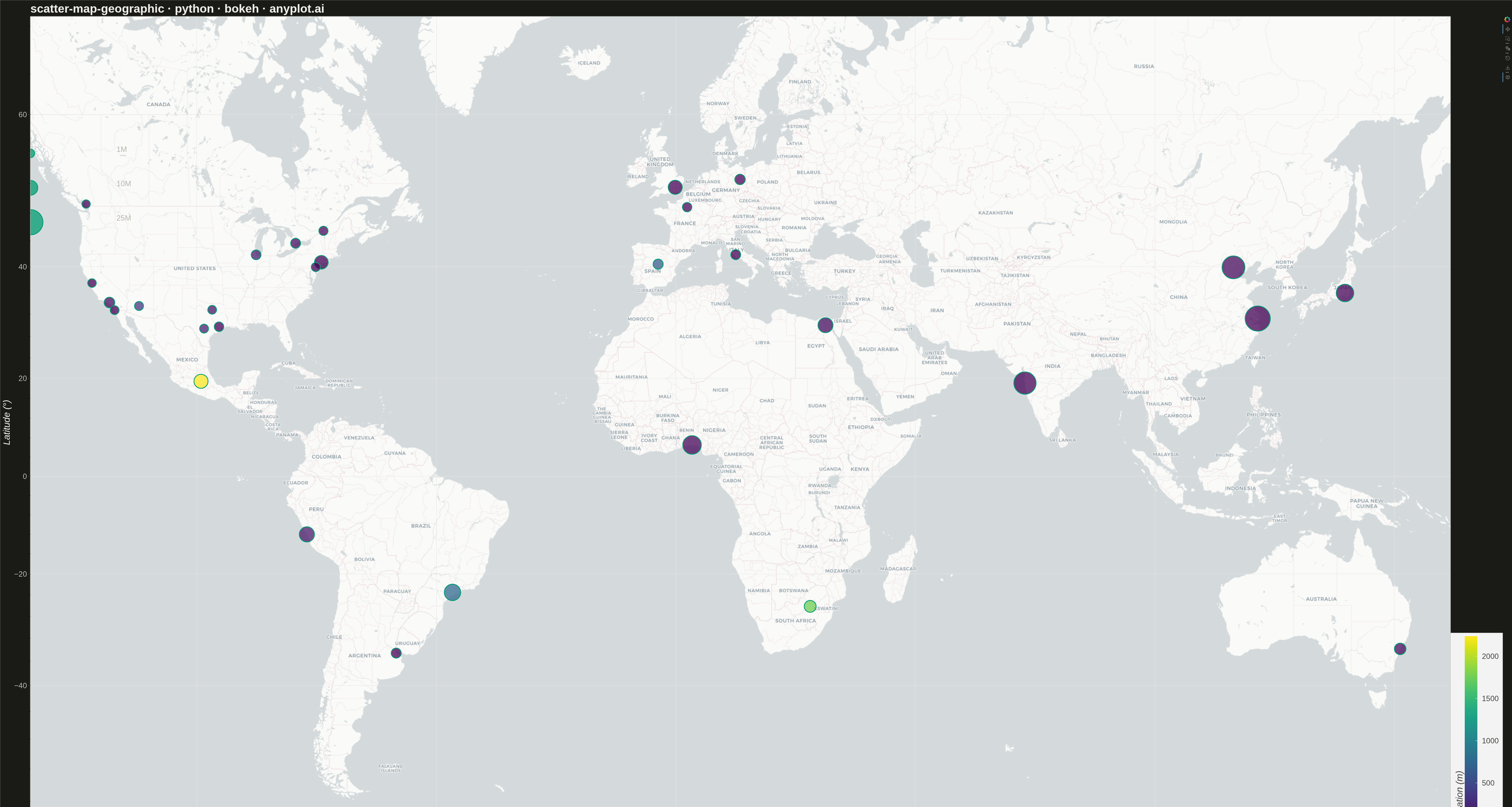
A geographic scatter plot that displays data points on a world or regional map, with each point positioned by its latitude and longitude coordinates. This visualization is ideal for showing spatial distributions of events, locations, or measurements across geographic areas. Points can optionally encode additional variables through size and color, enabling multi-dimensional geographic analysis at a glance.
""" anyplot.ai
scatter-map-geographic: Scatter Map with Geographic Points
Library: bokeh 3.9.0 | Python 3.13.13
Quality: 84/100 | Updated: 2026-05-18
"""

import os
import time
from pathlib import Path

import numpy as np
from bokeh.io import output_file, save
from bokeh.models import ColorBar, ColumnDataSource, LinearColorMapper, WMTSTileSource
from bokeh.plotting import figure
from selenium import webdriver
from selenium.webdriver.chrome.options import Options


# Theme tokens
THEME = os.getenv("ANYPLOT_THEME", "light")
PAGE_BG = "#FAF8F1" if THEME == "light" else "#1A1A17"
ELEVATED_BG = "#FFFDF6" if THEME == "light" else "#242420"
INK = "#1A1A17" if THEME == "light" else "#F0EFE8"
INK_SOFT = "#4A4A44" if THEME == "light" else "#B8B7B0"
BRAND = "#009E73"

# Data - Major cities with population and elevation
cities = {
    "name": [
        "New York",
        "Los Angeles",
        "Chicago",
        "Houston",
        "Phoenix",
        "Philadelphia",
        "San Antonio",
        "San Diego",
        "Dallas",
        "San Jose",
        "London",
        "Paris",
        "Berlin",
        "Madrid",
        "Rome",
        "Tokyo",
        "Beijing",
        "Shanghai",
        "Mumbai",
        "Sydney",
        "São Paulo",
        "Mexico City",
        "Cairo",
        "Lagos",
        "Johannesburg",
        "Toronto",
        "Vancouver",
        "Montreal",
        "Buenos Aires",
        "Lima",
    ],
    "lat": [
        40.71,
        34.05,
        41.88,
        29.76,
        33.45,
        39.95,
        29.42,
        32.72,
        32.78,
        37.34,
        51.51,
        48.86,
        52.52,
        40.42,
        41.90,
        35.68,
        39.90,
        31.23,
        19.08,
        -33.87,
        -23.55,
        19.43,
        30.04,
        6.52,
        -26.20,
        43.65,
        49.28,
        45.50,
        -34.60,
        -12.05,
    ],
    "lon": [
        -74.01,
        -118.24,
        -87.63,
        -95.37,
        -112.07,
        -75.17,
        -98.49,
        -117.16,
        -96.80,
        -121.89,
        -0.13,
        2.35,
        13.40,
        -3.70,
        12.50,
        139.69,
        116.41,
        121.47,
        72.88,
        151.21,
        -46.63,
        -99.13,
        31.24,
        3.38,
        28.04,
        -79.38,
        -123.12,
        -73.57,
        -58.38,
        -77.03,
    ],
    "population": [
        8.3,
        3.9,
        2.7,
        2.3,
        1.6,
        1.6,
        1.5,
        1.4,
        1.3,
        1.0,
        8.9,
        2.2,
        3.6,
        3.2,
        2.9,
        13.9,
        21.5,
        24.9,
        20.7,
        5.3,
        12.3,
        8.9,
        10.2,
        15.4,
        5.8,
        2.9,
        0.7,
        1.8,
        3.1,
        10.5,
    ],
    "elevation": [
        10,
        71,
        182,
        15,
        340,
        12,
        198,
        19,
        131,
        25,
        11,
        35,
        34,
        657,
        21,
        40,
        55,
        4,
        14,
        58,
        760,
        2240,
        75,
        41,
        1753,
        76,
        0,
        47,
        25,
        154,
    ],
}


# Convert lat/lon to Web Mercator projection (required for tile maps)
def lat_lon_to_mercator(lat, lon):
    k = 6378137
    x = lon * (k * np.pi / 180.0)
    y = np.log(np.tan((90 + lat) * np.pi / 360.0)) * k
    return x, y


lats = np.array(cities["lat"])
lons = np.array(cities["lon"])
mercator_x, mercator_y = lat_lon_to_mercator(lats, lons)

# Normalize size based on population (scaled for visibility on large canvas)
populations = np.array(cities["population"])
sizes = 25 + (populations / populations.max()) * 55

# Create color mapper for elevation
elevations = np.array(cities["elevation"])
color_mapper = LinearColorMapper(palette="Viridis256", low=elevations.min(), high=elevations.max())

# Create data source
source = ColumnDataSource(
    data={
        "x": mercator_x,
        "y": mercator_y,
        "name": cities["name"],
        "lat": lats,
        "lon": lons,
        "population": populations,
        "elevation": elevations,
        "size": sizes,
    }
)

# Create figure with tile map
p = figure(
    width=4800,
    height=2700,
    x_axis_type="mercator",
    y_axis_type="mercator",
    title="scatter-map-geographic · python · bokeh · anyplot.ai",
    tools="pan,wheel_zoom,box_zoom,reset,hover,save",
    tooltips=[
        ("City", "@name"),
        ("Population", "@population{0.0} million"),
        ("Elevation", "@elevation m"),
        ("Coordinates", "(@lat, @lon)"),
    ],
)

# Add map tiles
tile_url = "https://tiles.basemaps.cartocdn.com/light_all/{z}/{x}/{y}.png"
tile_source = WMTSTileSource(url=tile_url)
p.add_tile(tile_source)

# Add scatter points
p.scatter(
    x="x",
    y="y",
    source=source,
    size="size",
    fill_color={"field": "elevation", "transform": color_mapper},
    fill_alpha=0.75,
    line_color=BRAND,
    line_width=2.5,
)

# Add color bar for elevation
color_bar = ColorBar(
    color_mapper=color_mapper,
    title="Elevation (m)",
    title_text_font_size="22pt",
    major_label_text_font_size="18pt",
    label_standoff=15,
    border_line_color=INK_SOFT,
    location=(0, 0),
    width=40,
    height=600,
    margin=20,
)
p.add_layout(color_bar, "right")

# Add size legend for population by creating reference points

legend_items = [("1M", 1.0), ("10M", 10.0), ("25M", 24.9)]
legend_x_pos = -15000000
legend_y_start = 7500000
y_offset = 800000

for i, (label, pop) in enumerate(legend_items):
    size = 25 + (pop / populations.max()) * 55
    y = legend_y_start - (i * y_offset)
    p.scatter(x=[legend_x_pos], y=[y], size=size, fill_color=BRAND, fill_alpha=0.75, line_color=BRAND, line_width=2.5)
    p.text(x=[legend_x_pos + 2000000], y=[y], text=[label], text_font_size="18pt", text_color=INK_SOFT)

# Styling
p.title.text_font_size = "28pt"
p.title.text_color = INK
p.xaxis.axis_label = "Longitude (°)"
p.yaxis.axis_label = "Latitude (°)"
p.xaxis.axis_label_text_font_size = "22pt"
p.yaxis.axis_label_text_font_size = "22pt"
p.xaxis.major_label_text_font_size = "18pt"
p.yaxis.major_label_text_font_size = "18pt"
p.xaxis.axis_label_text_color = INK
p.yaxis.axis_label_text_color = INK
p.xaxis.major_label_text_color = INK_SOFT
p.yaxis.major_label_text_color = INK_SOFT
p.xaxis.axis_line_color = INK_SOFT
p.yaxis.axis_line_color = INK_SOFT
p.xaxis.major_tick_line_color = INK_SOFT
p.yaxis.major_tick_line_color = INK_SOFT

# Background and border
p.background_fill_color = PAGE_BG
p.border_fill_color = PAGE_BG
p.outline_line_color = INK_SOFT
p.outline_line_width = 2

# Set view to show entire world
p.x_range.start = -15000000
p.x_range.end = 18000000
p.y_range.start = -6000000
p.y_range.end = 8500000

# Save as interactive HTML
output_file(f"plot-{THEME}.html")
save(p)

# Screenshot with headless Chrome using Selenium
W, H = 4800, 2700
opts = Options()
for arg in (
    "--headless=new",
    "--no-sandbox",
    "--disable-dev-shm-usage",
    "--disable-gpu",
    f"--window-size={W},{H}",
    "--hide-scrollbars",
):
    opts.add_argument(arg)
driver = webdriver.Chrome(options=opts)
driver.set_window_size(W, H)
driver.get(f"file://{Path(f'plot-{THEME}.html').resolve()}")
time.sleep(3)
driver.save_screenshot(f"plot-{THEME}.png")
driver.quit()
Runnable source as JSON, for any HTTP client: https://api.anyplot.ai/specs/scatter-map-geographic/bokeh/code. Any spec id and library id listed in llms-full.txt fit the same URL shape; every URL below is complete and callable.
{
  "spec_id": "scatter-map-geographic",
  "language": "python",
  "library": "bokeh",
  "page": "https://anyplot.ai/scatter-map-geographic/python/bokeh",
  "hub": "https://anyplot.ai/scatter-map-geographic",
  "code_json": "https://api.anyplot.ai/specs/scatter-map-geographic/bokeh/code",
  "spec_json": "https://api.anyplot.ai/specs/scatter-map-geographic",
  "render_light_png": "https://storage.googleapis.com/anyplot-images/plots/scatter-map-geographic/python/bokeh/plot-light.png",
  "render_dark_png": "https://storage.googleapis.com/anyplot-images/plots/scatter-map-geographic/python/bokeh/plot-dark.png",
  "interactive_light_html": "https://storage.googleapis.com/anyplot-images/plots/scatter-map-geographic/python/bokeh/plot-light.html",
  "interactive_dark_html": "https://storage.googleapis.com/anyplot-images/plots/scatter-map-geographic/python/bokeh/plot-dark.html",
  "quality_score": 84.0,
  "license": "MIT",
  "guide": "https://anyplot.ai/llms.txt"
}
Part of Scatter Map with Geographic Points on anyplot.ai.