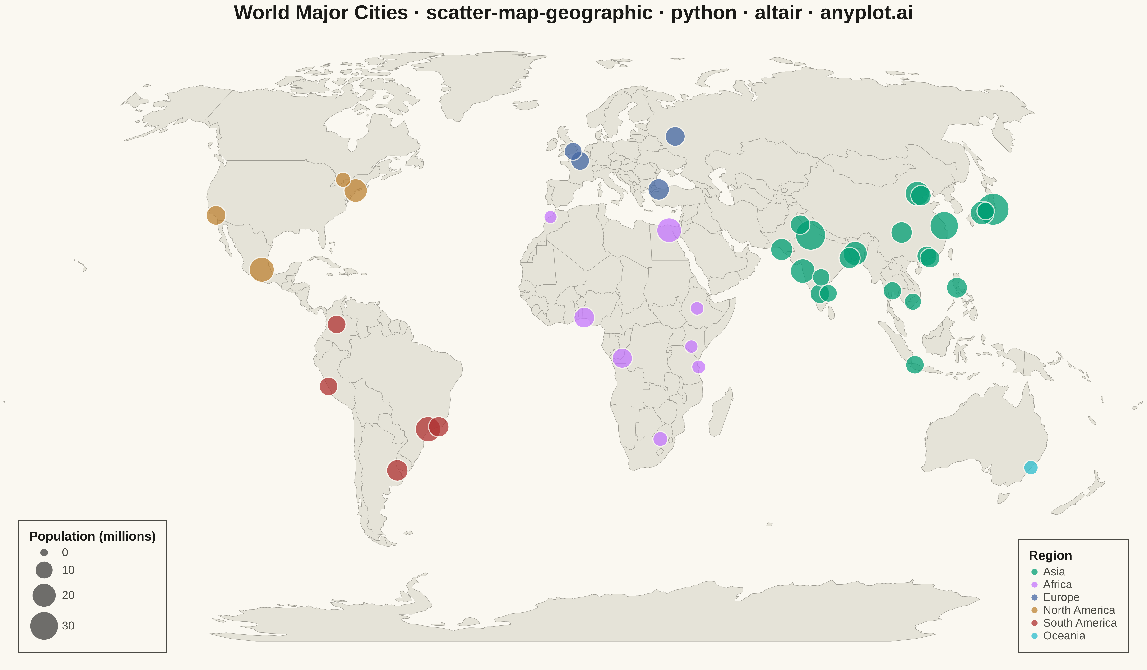
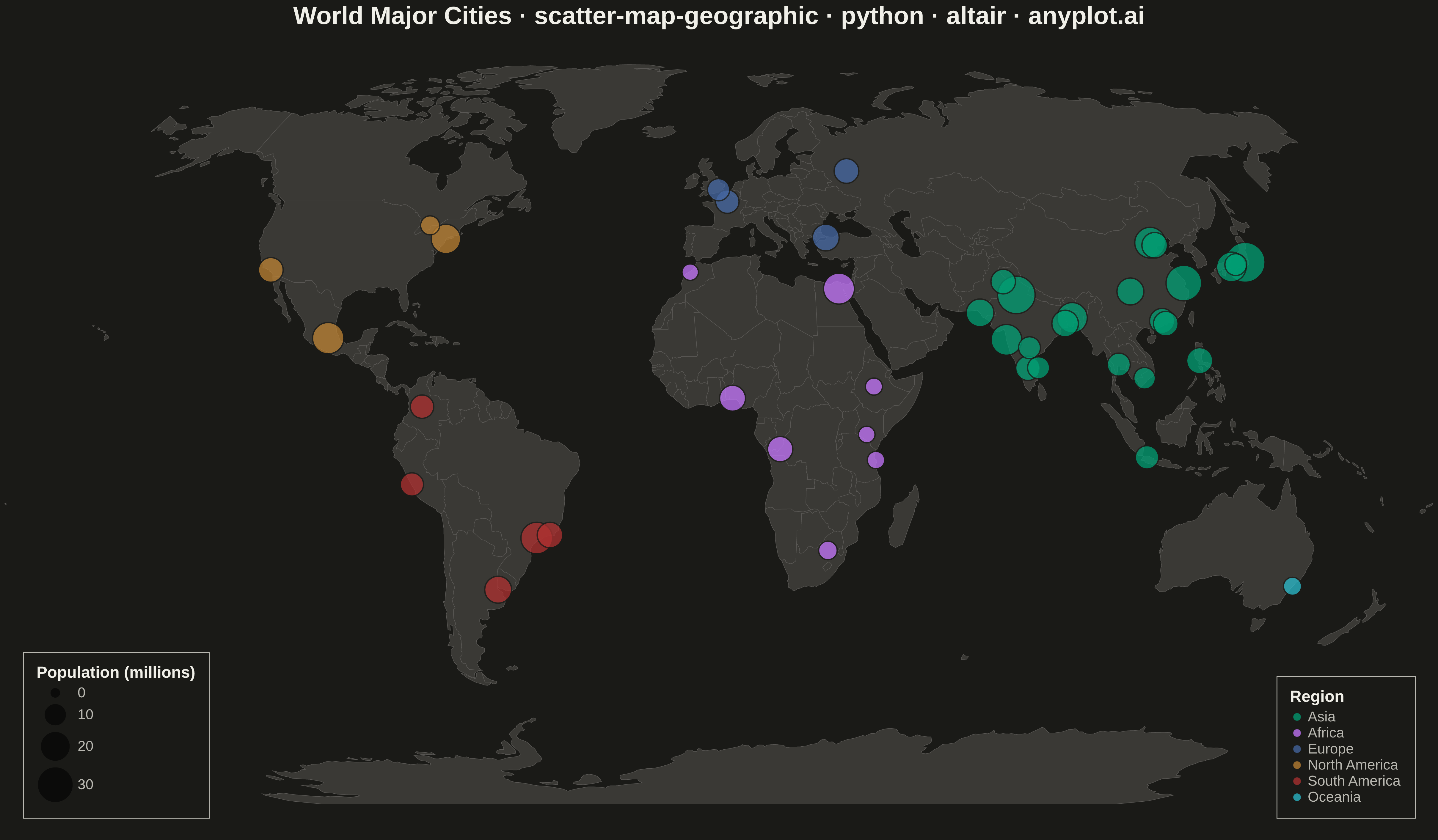
A geographic scatter plot that displays data points on a world or regional map, with each point positioned by its latitude and longitude coordinates. This visualization is ideal for showing spatial distributions of events, locations, or measurements across geographic areas. Points can optionally encode additional variables through size and color, enabling multi-dimensional geographic analysis at a glance.
""" anyplot.ai
scatter-map-geographic: Scatter Map with Geographic Points
Library: altair 6.1.0 | Python 3.13.13
Quality: 94/100 | Updated: 2026-05-18
"""

import os
import sys


script_dir = os.path.dirname(os.path.abspath(__file__))
while script_dir in sys.path:
    sys.path.remove(script_dir)

import altair as alt
import pandas as pd


# Theme tokens
THEME = os.getenv("ANYPLOT_THEME", "light")
PAGE_BG = "#FAF8F1" if THEME == "light" else "#1A1A17"
INK = "#1A1A17" if THEME == "light" else "#F0EFE8"
INK_SOFT = "#4A4A44" if THEME == "light" else "#B8B7B0"
BASEMAP_FILL = "#E5E3D8" if THEME == "light" else "#3A3935"
BASEMAP_STROKE = "#9C9A91" if THEME == "light" else "#5A5855"

# Data: Major world cities with population and region
cities_data = {
    "city": [
        "Tokyo",
        "Delhi",
        "Shanghai",
        "São Paulo",
        "Mexico City",
        "Cairo",
        "Mumbai",
        "Beijing",
        "Dhaka",
        "Osaka",
        "New York",
        "Karachi",
        "Buenos Aires",
        "Chongqing",
        "Istanbul",
        "Kolkata",
        "Manila",
        "Lagos",
        "Rio de Janeiro",
        "Tianjin",
        "Kinshasa",
        "Guangzhou",
        "Los Angeles",
        "Moscow",
        "Shenzhen",
        "Lahore",
        "Bangalore",
        "Paris",
        "Bogotá",
        "Jakarta",
        "Lima",
        "Bangkok",
        "London",
        "Chennai",
        "Hyderabad",
        "Nagoya",
        "Ho Chi Minh City",
        "Johannesburg",
        "Toronto",
        "Sydney",
        "Casablanca",
        "Addis Ababa",
        "Nairobi",
        "Dar es Salaam",
    ],
    "latitude": [
        35.6762,
        28.7041,
        31.2304,
        -23.5505,
        19.4326,
        30.0444,
        19.0760,
        39.9042,
        23.8103,
        34.6937,
        40.7128,
        24.8607,
        -34.6037,
        29.4316,
        41.0082,
        22.5726,
        14.5995,
        6.5244,
        -22.9068,
        39.3434,
        -4.4419,
        23.1291,
        34.0522,
        55.7558,
        22.5431,
        31.5497,
        12.9716,
        48.8566,
        4.7110,
        -6.2088,
        -12.0464,
        13.7563,
        51.5074,
        13.0827,
        17.3850,
        35.1815,
        10.8231,
        -26.2041,
        43.6532,
        -33.8688,
        33.5731,
        9.0320,
        -1.2921,
        -6.8000,
    ],
    "longitude": [
        139.6503,
        77.1025,
        121.4737,
        -46.6333,
        -99.1332,
        31.2357,
        72.8777,
        116.4074,
        90.4125,
        135.5023,
        -74.0060,
        67.0011,
        -58.3816,
        106.9123,
        28.9784,
        88.3639,
        120.9842,
        3.3792,
        -43.1729,
        117.3616,
        15.2663,
        113.2644,
        -118.2437,
        37.6173,
        114.0579,
        74.3436,
        77.5946,
        2.3522,
        -74.0721,
        106.8456,
        -77.0428,
        100.5018,
        -0.1278,
        80.2707,
        78.4867,
        136.9066,
        106.6297,
        28.0473,
        -79.3832,
        151.2093,
        -7.5898,
        38.7469,
        36.8219,
        39.2069,
    ],
    "population_millions": [
        37.4,
        32.9,
        29.2,
        22.4,
        21.9,
        21.3,
        21.0,
        20.9,
        20.3,
        19.2,
        18.8,
        16.5,
        15.4,
        15.4,
        15.2,
        14.9,
        14.2,
        14.1,
        13.6,
        13.6,
        13.2,
        13.0,
        12.5,
        12.5,
        12.4,
        12.3,
        12.2,
        11.0,
        10.9,
        10.8,
        10.7,
        10.5,
        9.5,
        9.3,
        9.2,
        9.1,
        8.8,
        5.8,
        6.2,
        5.3,
        3.9,
        4.4,
        4.0,
        4.7,
    ],
    "region": [
        "Asia",
        "Asia",
        "Asia",
        "South America",
        "North America",
        "Africa",
        "Asia",
        "Asia",
        "Asia",
        "Asia",
        "North America",
        "Asia",
        "South America",
        "Asia",
        "Europe",
        "Asia",
        "Asia",
        "Africa",
        "South America",
        "Asia",
        "Africa",
        "Asia",
        "North America",
        "Europe",
        "Asia",
        "Asia",
        "Asia",
        "Europe",
        "South America",
        "Asia",
        "South America",
        "Asia",
        "Europe",
        "Asia",
        "Asia",
        "Asia",
        "Asia",
        "Africa",
        "North America",
        "Oceania",
        "Africa",
        "Africa",
        "Africa",
        "Africa",
    ],
}

df = pd.DataFrame(cities_data)

# Load world basemap
world = alt.topo_feature("https://cdn.jsdelivr.net/npm/world-atlas@2/countries-110m.json", "countries")

# Create basemap layer
basemap = (
    alt.Chart(world)
    .mark_geoshape(fill=BASEMAP_FILL, stroke=BASEMAP_STROKE, strokeWidth=0.5)
    .project(type="naturalEarth1")
    .properties(width=1600, height=900)
)

# Define color scale for regions using Okabe-Ito palette positions
region_colors = {
    "Asia": "#009E73",  # OI position 1 (brand green)
    "Africa": "#C475FD",  # OI position 2 (vermillion)
    "Europe": "#4467A3",  # OI position 3 (blue)
    "North America": "#BD8233",  # OI position 4 (reddish purple)
    "South America": "#AE3030",  # OI position 5 (orange)
    "Oceania": "#2ABCCD",  # OI position 6 (sky blue)
}

# Create scatter points layer
points = (
    alt.Chart(df)
    .mark_circle(opacity=0.75, stroke=PAGE_BG, strokeWidth=1.5)
    .encode(
        longitude="longitude:Q",
        latitude="latitude:Q",
        size=alt.Size(
            "population_millions:Q",
            scale=alt.Scale(range=[150, 2000]),
            legend=alt.Legend(
                title="Population (millions)", titleFontSize=18, labelFontSize=16, orient="bottom-left", offset=20
            ),
        ),
        color=alt.Color(
            "region:N",
            scale=alt.Scale(domain=list(region_colors.keys()), range=list(region_colors.values())),
            legend=alt.Legend(title="Region", titleFontSize=18, labelFontSize=16, orient="bottom-right", offset=20),
        ),
        tooltip=["city:N", "population_millions:Q", "region:N"],
    )
    .project(type="naturalEarth1")
    .properties(width=1600, height=900)
)

# Combine layers with theme-adaptive styling
chart = (
    alt.layer(basemap, points)
    .properties(
        title=alt.Title(
            text="World Major Cities · scatter-map-geographic · python · altair · anyplot.ai",
            fontSize=28,
            anchor="middle",
            color=INK,
        ),
        background=PAGE_BG,
    )
    .configure_view(stroke=None, fill=PAGE_BG)
    .configure_legend(
        padding=15,
        cornerRadius=0,
        fillColor="transparent",
        strokeColor=INK_SOFT,
        strokeWidth=1,
        labelColor=INK_SOFT,
        titleColor=INK,
    )
    .configure_axis(labelColor=INK_SOFT, titleColor=INK)
    .configure_title(color=INK)
)

# Save as PNG and HTML with theme-suffixed filenames
script_dir = os.path.dirname(os.path.abspath(__file__))
png_path = os.path.join(script_dir, f"plot-{THEME}.png")
html_path = os.path.join(script_dir, f"plot-{THEME}.html")
chart.save(png_path, scale_factor=3.0)
chart.save(html_path)
Runnable source as JSON, for any HTTP client: https://api.anyplot.ai/specs/scatter-map-geographic/altair/code. Any spec id and library id listed in llms-full.txt fit the same URL shape; every URL below is complete and callable.
{
  "spec_id": "scatter-map-geographic",
  "language": "python",
  "library": "altair",
  "page": "https://anyplot.ai/scatter-map-geographic/python/altair",
  "hub": "https://anyplot.ai/scatter-map-geographic",
  "code_json": "https://api.anyplot.ai/specs/scatter-map-geographic/altair/code",
  "spec_json": "https://api.anyplot.ai/specs/scatter-map-geographic",
  "render_light_png": "https://storage.googleapis.com/anyplot-images/plots/scatter-map-geographic/python/altair/plot-light.png",
  "render_dark_png": "https://storage.googleapis.com/anyplot-images/plots/scatter-map-geographic/python/altair/plot-dark.png",
  "interactive_light_html": "https://storage.googleapis.com/anyplot-images/plots/scatter-map-geographic/python/altair/plot-light.html",
  "interactive_dark_html": "https://storage.googleapis.com/anyplot-images/plots/scatter-map-geographic/python/altair/plot-dark.html",
  "quality_score": 94.0,
  "license": "MIT",
  "guide": "https://anyplot.ai/llms.txt"
}
Part of Scatter Map with Geographic Points on anyplot.ai.