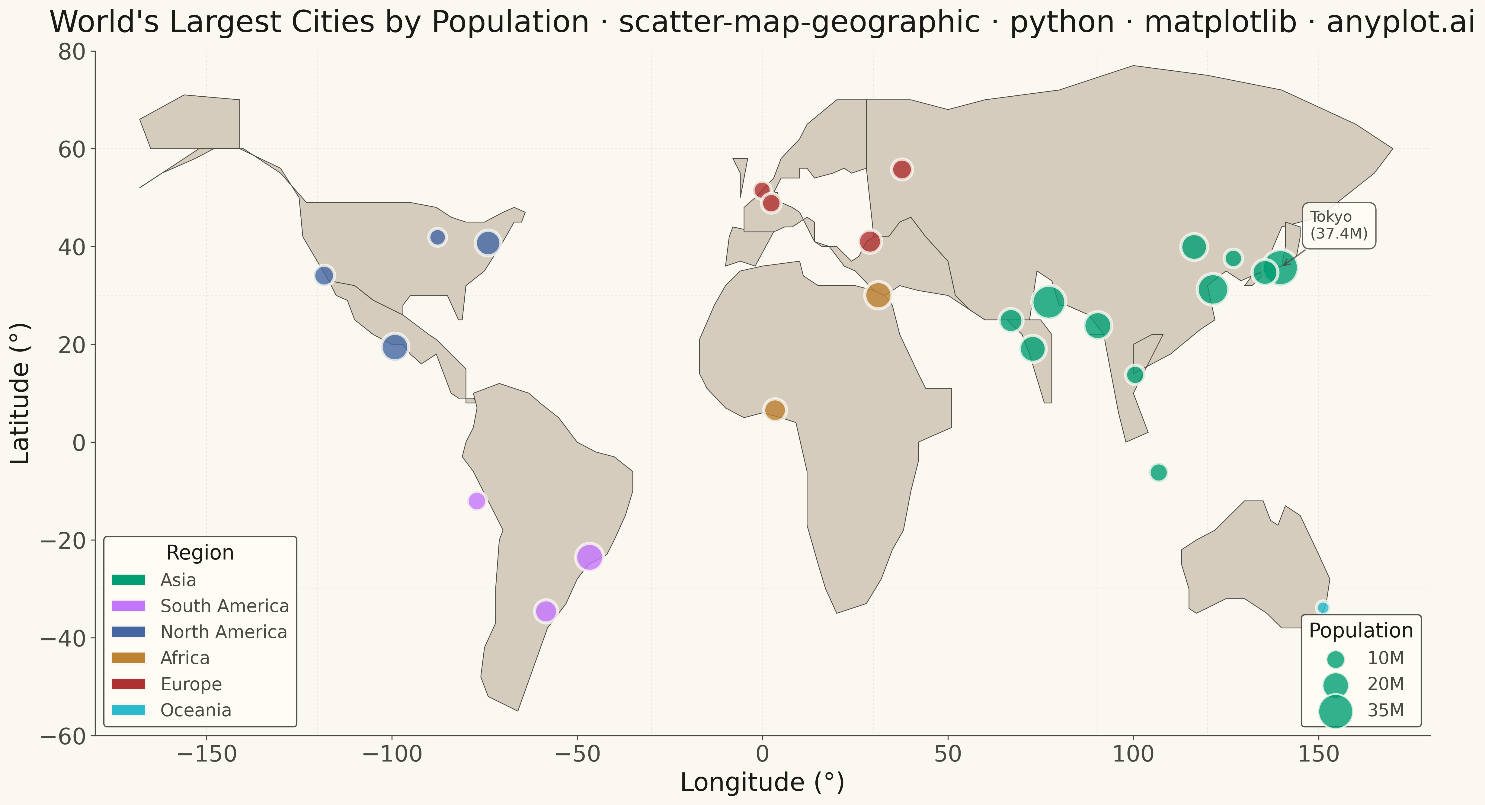
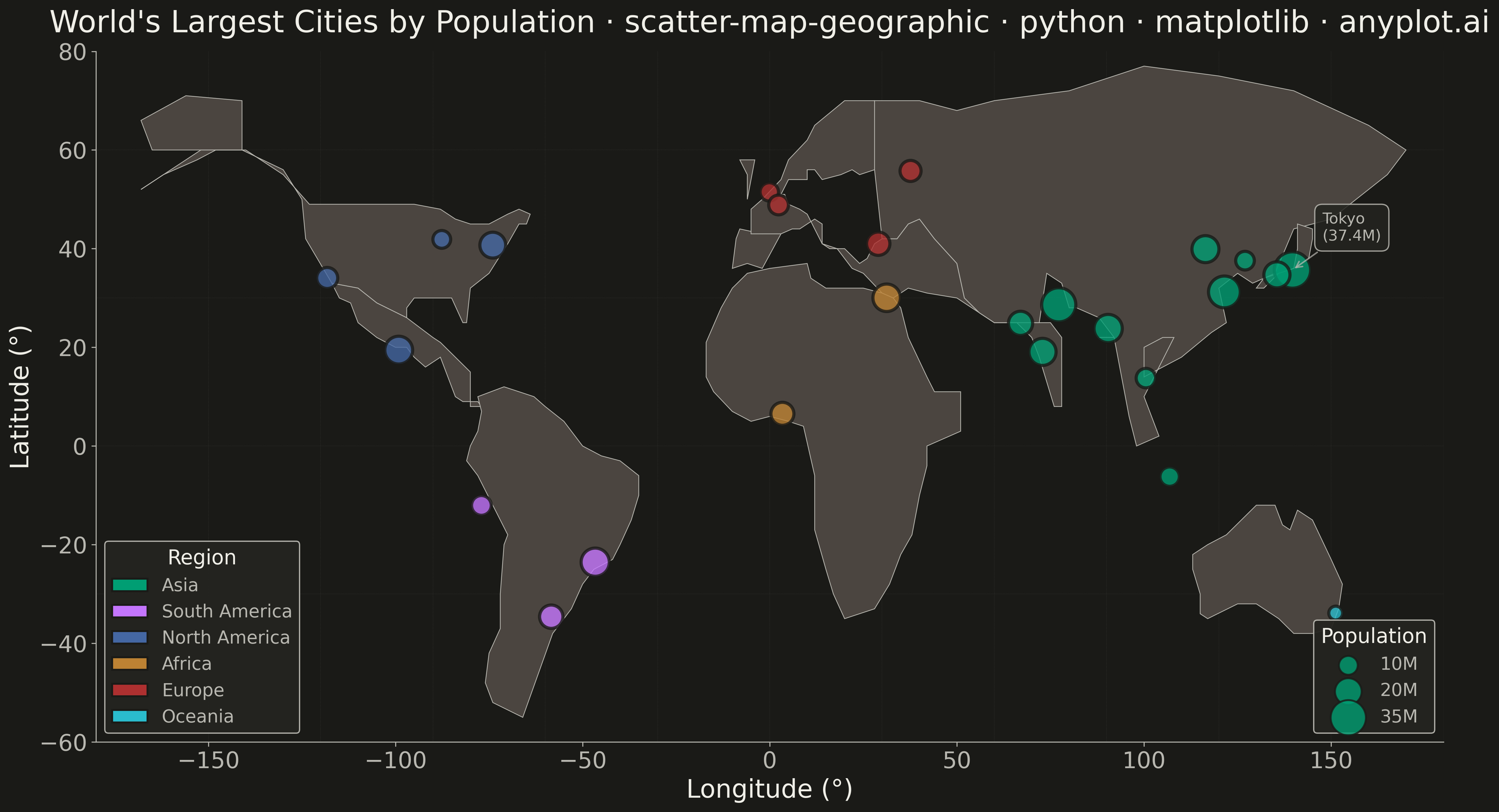
A geographic scatter plot that displays data points on a world or regional map, with each point positioned by its latitude and longitude coordinates. This visualization is ideal for showing spatial distributions of events, locations, or measurements across geographic areas. Points can optionally encode additional variables through size and color, enabling multi-dimensional geographic analysis at a glance.
""" anyplot.ai
scatter-map-geographic: Scatter Map with Geographic Points
Library: matplotlib 3.10.9 | Python 3.13.13
Quality: 95/100 | Updated: 2026-05-18
"""

import os

import matplotlib.patches as mpatches
import matplotlib.pyplot as plt
import numpy as np


# Theme tokens
THEME = os.getenv("ANYPLOT_THEME", "light")
PAGE_BG = "#FAF8F1" if THEME == "light" else "#1A1A17"
ELEVATED_BG = "#FFFDF6" if THEME == "light" else "#242420"
INK = "#1A1A17" if THEME == "light" else "#F0EFE8"
INK_SOFT = "#4A4A44" if THEME == "light" else "#B8B7B0"
INK_MUTED = "#6B6A63" if THEME == "light" else "#A8A79F"

# Okabe-Ito palette — use positions 1→N in canonical order
IMPRINT = [
    "#009E73",  # 1: bluish green (ALWAYS first series)
    "#C475FD",  # 2: vermillion
    "#4467A3",  # 3: blue
    "#BD8233",  # 4: reddish purple
    "#AE3030",  # 5: orange
    "#2ABCCD",  # 6: sky blue
]

# Data - Major world cities with population and region
np.random.seed(42)

cities = {
    "Tokyo": (35.6762, 139.6503, 37.4, "Asia"),
    "Delhi": (28.6139, 77.2090, 32.9, "Asia"),
    "Shanghai": (31.2304, 121.4737, 28.5, "Asia"),
    "São Paulo": (-23.5505, -46.6333, 22.4, "South America"),
    "Mexico City": (19.4326, -99.1332, 21.8, "North America"),
    "Cairo": (30.0444, 31.2357, 21.3, "Africa"),
    "Mumbai": (19.0760, 72.8777, 20.7, "Asia"),
    "Beijing": (39.9042, 116.4074, 20.5, "Asia"),
    "Dhaka": (23.8103, 90.4125, 22.5, "Asia"),
    "Osaka": (34.6937, 135.5023, 19.2, "Asia"),
    "New York": (40.7128, -74.0060, 18.8, "North America"),
    "Karachi": (24.8607, 67.0011, 16.5, "Asia"),
    "Buenos Aires": (-34.6037, -58.3816, 15.4, "South America"),
    "Istanbul": (41.0082, 28.9784, 15.4, "Europe"),
    "Lagos": (6.5244, 3.3792, 14.9, "Africa"),
    "Los Angeles": (34.0522, -118.2437, 12.5, "North America"),
    "London": (51.5074, -0.1278, 9.5, "Europe"),
    "Paris": (48.8566, 2.3522, 11.0, "Europe"),
    "Moscow": (55.7558, 37.6173, 12.5, "Europe"),
    "Chicago": (41.8781, -87.6298, 8.9, "North America"),
    "Sydney": (-33.8688, 151.2093, 5.4, "Oceania"),
    "Lima": (-12.0464, -77.0428, 11.0, "South America"),
    "Bangkok": (13.7563, 100.5018, 10.7, "Asia"),
    "Seoul": (37.5665, 126.9780, 9.8, "Asia"),
    "Jakarta": (-6.2088, 106.8456, 10.6, "Asia"),
}

# Extract data
names = list(cities.keys())
lats = np.array([cities[c][0] for c in names])
lons = np.array([cities[c][1] for c in names])
populations = np.array([cities[c][2] for c in names])
regions = [cities[c][3] for c in names]

# Map regions to Okabe-Ito colors
unique_regions = ["Asia", "South America", "North America", "Africa", "Europe", "Oceania"]
region_colors = {region: IMPRINT[i] for i, region in enumerate(unique_regions)}
colors = [region_colors[r] for r in regions]

# Scale sizes based on population
sizes = populations * 22

# Simplified world map coastlines
continents = [
    # North America
    [(-168, 66), (-165, 60), (-141, 60), (-141, 70), (-156, 71), (-168, 66)],
    # Alaska + Canada + USA main
    [
        (-168, 52),
        (-162, 55),
        (-152, 60),
        (-141, 60),
        (-130, 56),
        (-125, 50),
        (-124, 42),
        (-117, 33),
        (-110, 32),
        (-105, 29),
        (-97, 26),
        (-97, 28),
        (-95, 30),
        (-90, 30),
        (-85, 30),
        (-82, 25),
        (-81, 25),
        (-80, 32),
        (-75, 35),
        (-70, 41),
        (-67, 45),
        (-65, 45),
        (-64, 47),
        (-67, 48),
        (-70, 47),
        (-75, 45),
        (-80, 45),
        (-84, 46),
        (-88, 48),
        (-95, 49),
        (-102, 49),
        (-120, 49),
        (-123, 49),
        (-130, 55),
        (-140, 60),
        (-148, 60),
        (-153, 58),
        (-162, 55),
        (-168, 52),
    ],
    # Mexico + Central America
    [
        (-117, 33),
        (-115, 30),
        (-112, 29),
        (-110, 25),
        (-105, 22),
        (-100, 20),
        (-97, 20),
        (-95, 18),
        (-92, 16),
        (-88, 18),
        (-87, 16),
        (-84, 10),
        (-82, 9),
        (-78, 9),
        (-77, 8),
        (-80, 8),
        (-80, 15),
        (-88, 21),
        (-90, 22),
        (-97, 26),
        (-105, 29),
        (-110, 32),
        (-117, 33),
    ],
    # South America
    [
        (-78, 10),
        (-71, 12),
        (-67, 11),
        (-63, 10),
        (-60, 8),
        (-55, 5),
        (-50, 0),
        (-45, -2),
        (-40, -3),
        (-35, -6),
        (-35, -10),
        (-37, -15),
        (-40, -20),
        (-42, -23),
        (-47, -25),
        (-50, -28),
        (-53, -33),
        (-58, -38),
        (-66, -55),
        (-74, -52),
        (-76, -48),
        (-75, -42),
        (-72, -37),
        (-72, -30),
        (-71, -20),
        (-70, -18),
        (-78, -6),
        (-81, -3),
        (-80, 0),
        (-78, 3),
        (-77, 7),
        (-78, 10),
    ],
    # Europe + UK
    [(-10, 36), (-6, 37), (-2, 36), (3, 43), (0, 44), (-2, 43), (-8, 44), (-9, 42), (-10, 36)],
    [(-6, 50), (-5, 54), (-4, 58), (-8, 58), (-6, 55), (-6, 50)],
    # European mainland
    [
        (-5, 43),
        (0, 43),
        (3, 43),
        (6, 44),
        (8, 44),
        (12, 46),
        (14, 45),
        (14, 41),
        (16, 40),
        (20, 40),
        (24, 37),
        (26, 38),
        (28, 41),
        (30, 42),
        (32, 42),
        (34, 42),
        (37, 45),
        (40, 46),
        (44, 42),
        (50, 37),
        (52, 30),
        (56, 27),
        (60, 25),
        (70, 25),
        (75, 25),
        (78, 22),
        (78, 8),
        (76, 8),
        (72, 18),
        (70, 22),
        (66, 25),
        (60, 25),
        (56, 27),
        (50, 30),
        (42, 31),
        (37, 32),
        (33, 30),
        (30, 31),
        (25, 35),
        (22, 36),
        (18, 40),
        (14, 41),
        (12, 44),
        (10, 47),
        (8, 48),
        (5, 49),
        (4, 51),
        (3, 51),
        (5, 54),
        (10, 54),
        (10, 56),
        (12, 56),
        (14, 54),
        (19, 55),
        (22, 56),
        (24, 55),
        (28, 56),
        (30, 60),
        (32, 65),
        (28, 70),
        (20, 70),
        (12, 65),
        (10, 62),
        (5, 58),
        (3, 54),
        (-2, 50),
        (-5, 48),
        (-5, 43),
    ],
    # Africa
    [
        (-17, 14),
        (-17, 21),
        (-13, 28),
        (-10, 32),
        (-6, 35),
        (0, 36),
        (10, 37),
        (11, 34),
        (15, 32),
        (20, 32),
        (25, 32),
        (30, 31),
        (33, 30),
        (35, 28),
        (37, 22),
        (42, 14),
        (44, 11),
        (51, 11),
        (51, 3),
        (42, 0),
        (42, -4),
        (40, -10),
        (38, -18),
        (35, -22),
        (32, -28),
        (28, -33),
        (20, -35),
        (17, -30),
        (15, -25),
        (12, -17),
        (12, -6),
        (9, 4),
        (5, 5),
        (0, 6),
        (-5, 5),
        (-10, 7),
        (-15, 11),
        (-17, 14),
    ],
    # Asia (main landmass - simplified)
    [
        (28, 70),
        (40, 70),
        (50, 68),
        (60, 70),
        (80, 72),
        (100, 77),
        (120, 75),
        (140, 72),
        (160, 65),
        (170, 60),
        (165, 55),
        (160, 52),
        (150, 46),
        (140, 44),
        (135, 35),
        (129, 33),
        (125, 35),
        (120, 32),
        (122, 25),
        (118, 23),
        (110, 18),
        (105, 16),
        (100, 14),
        (100, 20),
        (105, 22),
        (108, 22),
        (100, 10),
        (104, 2),
        (98, 0),
        (96, 6),
        (92, 22),
        (88, 22),
        (92, 22),
        (88, 26),
        (82, 28),
        (80, 28),
        (78, 33),
        (74, 35),
        (72, 25),
        (66, 25),
        (60, 25),
        (56, 27),
        (52, 30),
        (50, 37),
        (44, 42),
        (40, 46),
        (37, 45),
        (34, 42),
        (32, 42),
        (30, 42),
        (28, 56),
        (28, 70),
    ],
    # Japan
    [
        (130, 32),
        (132, 34),
        (136, 35),
        (140, 36),
        (141, 40),
        (141, 45),
        (145, 44),
        (145, 42),
        (144, 38),
        (140, 36),
        (136, 35),
        (132, 32),
        (130, 32),
    ],
    # Australia
    [
        (113, -22),
        (115, -21),
        (117, -20),
        (122, -18),
        (130, -12),
        (135, -12),
        (137, -16),
        (139, -17),
        (141, -13),
        (145, -15),
        (150, -23),
        (153, -28),
        (152, -33),
        (150, -37),
        (145, -38),
        (140, -38),
        (136, -35),
        (130, -32),
        (125, -32),
        (117, -35),
        (115, -34),
        (115, -30),
        (113, -25),
        (113, -22),
    ],
]

# Plot
fig, ax = plt.subplots(figsize=(16, 9), facecolor=PAGE_BG)
ax.set_facecolor(PAGE_BG)

# Ocean color (theme-adaptive) - sophisticated water tones
ocean_bg = "#C5D9ED" if THEME == "light" else "#3A4E68"

# Draw continents (theme-adaptive) - refined earth tones
continent_color = "#D6CCBE" if THEME == "light" else "#4B4540"
continent_edge = INK_SOFT
for continent in continents:
    poly = plt.Polygon(continent, facecolor=continent_color, edgecolor=continent_edge, linewidth=0.6, zorder=1)
    ax.add_patch(poly)

# Add graticule (grid lines)
for lat in range(-60, 90, 30):
    ax.axhline(y=lat, color=INK_SOFT, linewidth=0.4, linestyle=":", alpha=0.15, zorder=0)
for lon in range(-150, 181, 30):
    ax.axvline(x=lon, color=INK_SOFT, linewidth=0.4, linestyle=":", alpha=0.15, zorder=0)

# Plot cities
ax.scatter(lons, lats, c=colors, s=sizes, alpha=0.8, edgecolors=PAGE_BG, linewidths=2.5, zorder=5)

# Highlight Tokyo with subtle annotation for visual storytelling
tokyo_lat, tokyo_lon = 35.6762, 139.6503
ax.annotate(
    "Tokyo\n(37.4M)",
    xy=(tokyo_lon, tokyo_lat),
    xytext=(tokyo_lon + 8, tokyo_lat + 6),
    fontsize=12,
    color=INK_SOFT,
    weight="medium",
    bbox={"boxstyle": "round,pad=0.5", "facecolor": ELEVATED_BG, "edgecolor": INK_SOFT, "alpha": 0.85},
    arrowprops={"arrowstyle": "->", "color": INK_SOFT, "lw": 1.2, "alpha": 0.7},
    zorder=10,
)

# Set axis limits
ax.set_xlim(-180, 180)
ax.set_ylim(-60, 80)

# Style
ax.set_xlabel("Longitude (°)", fontsize=20, color=INK)
ax.set_ylabel("Latitude (°)", fontsize=20, color=INK)
ax.set_title(
    "World's Largest Cities by Population · scatter-map-geographic · python · matplotlib · anyplot.ai",
    fontsize=24,
    fontweight="medium",
    color=INK,
    pad=15,
)
ax.tick_params(axis="both", labelsize=18, colors=INK_SOFT)
for s in ("left", "bottom"):
    ax.spines[s].set_color(INK_SOFT)
ax.spines["top"].set_visible(False)
ax.spines["right"].set_visible(False)

# Create region legend
legend_handles = []
for region in unique_regions:
    color = region_colors[region]
    handle = mpatches.Patch(facecolor=color, edgecolor=PAGE_BG, linewidth=1.5, label=region)
    legend_handles.append(handle)

region_legend = ax.legend(
    handles=legend_handles,
    title="Region",
    loc="lower left",
    fontsize=14,
    title_fontsize=16,
    framealpha=0.95,
    facecolor=ELEVATED_BG,
    edgecolor=INK_SOFT,
)
region_legend.get_title().set_color(INK)
plt.setp(region_legend.get_texts(), color=INK_SOFT)
ax.add_artist(region_legend)

# Create size legend (population)
size_values = [10, 20, 35]
size_labels = ["10M", "20M", "35M"]
size_handles = []
for val, label in zip(size_values, size_labels, strict=True):
    handle = ax.scatter([], [], c=IMPRINT[0], s=val * 22, label=label, edgecolors=PAGE_BG, linewidths=1.5, alpha=0.8)
    size_handles.append(handle)

size_legend = ax.legend(
    handles=size_handles,
    title="Population",
    loc="lower right",
    fontsize=14,
    title_fontsize=16,
    framealpha=0.95,
    facecolor=ELEVATED_BG,
    edgecolor=INK_SOFT,
)
size_legend.get_title().set_color(INK)
plt.setp(size_legend.get_texts(), color=INK_SOFT)

plt.tight_layout()
plt.savefig(f"plot-{THEME}.png", dpi=300, bbox_inches="tight", facecolor=PAGE_BG)
Runnable source as JSON, for any HTTP client: https://api.anyplot.ai/specs/scatter-map-geographic/matplotlib/code. Any spec id and library id listed in llms-full.txt fit the same URL shape; every URL below is complete and callable.
{
  "spec_id": "scatter-map-geographic",
  "language": "python",
  "library": "matplotlib",
  "page": "https://anyplot.ai/scatter-map-geographic/python/matplotlib",
  "hub": "https://anyplot.ai/scatter-map-geographic",
  "code_json": "https://api.anyplot.ai/specs/scatter-map-geographic/matplotlib/code",
  "spec_json": "https://api.anyplot.ai/specs/scatter-map-geographic",
  "render_light_png": "https://storage.googleapis.com/anyplot-images/plots/scatter-map-geographic/python/matplotlib/plot-light.png",
  "render_dark_png": "https://storage.googleapis.com/anyplot-images/plots/scatter-map-geographic/python/matplotlib/plot-dark.png",
  "quality_score": 95.0,
  "license": "MIT",
  "guide": "https://anyplot.ai/llms.txt"
}
Part of Scatter Map with Geographic Points on anyplot.ai.