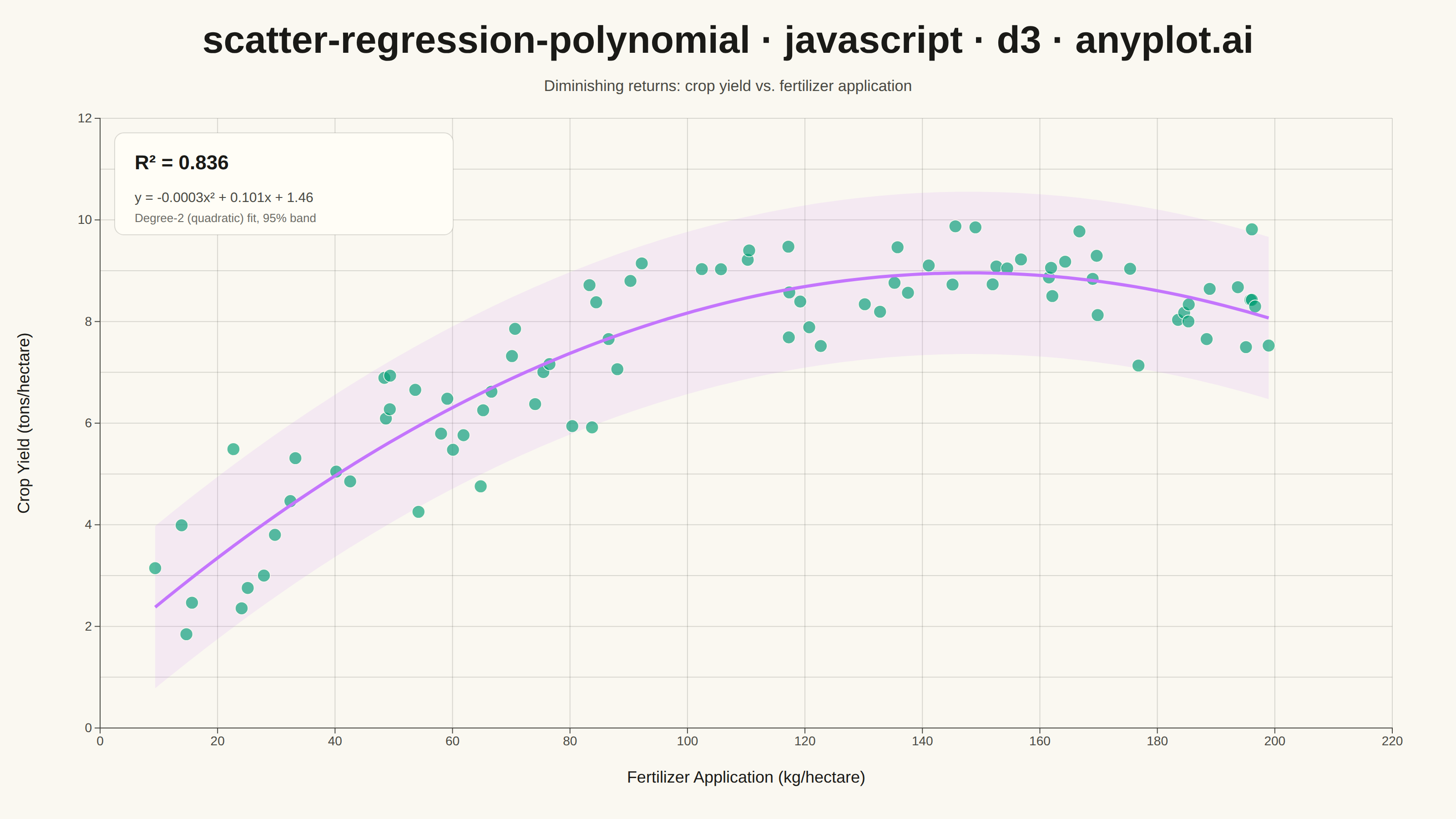
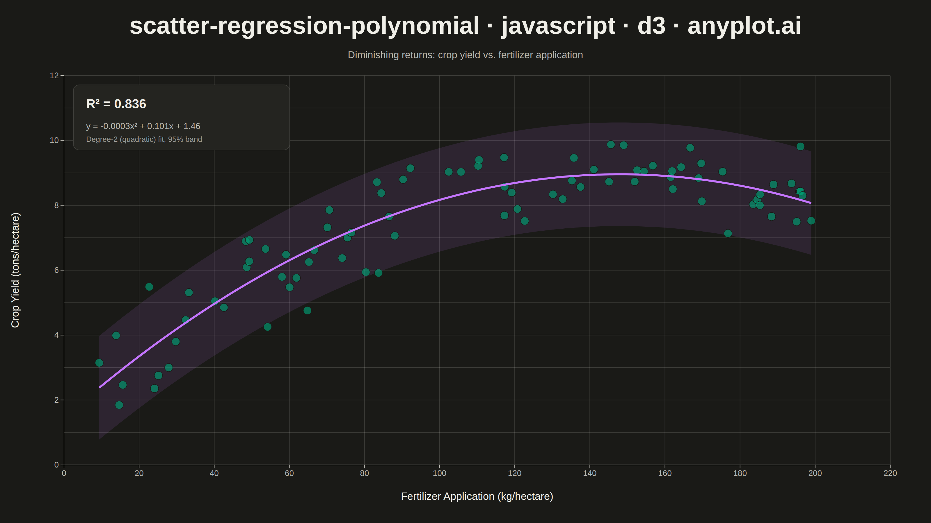
The same plot in 14 other libraries — JavaScript: Chart.js, Apache ECharts, Highcharts, MUI X Charts; Python: Altair, Bokeh, lets-plot, Matplotlib, Plotly, plotnine, Pygal, Seaborn; R: ggplot2; Julia: Makie.jl. Compare all 15 side by side: Scatter Plot with Polynomial Regression in Python, R, Julia and JavaScript.
A scatter plot displaying the relationship between two numeric variables with a fitted polynomial regression curve (degree 2-4). This visualization extends beyond linear regression to capture non-linear relationships in data, making it ideal for modeling curved trends, parabolic patterns, and complex data relationships where a straight line would not adequately represent the underlying pattern.
// anyplot.ai
// scatter-regression-polynomial: Scatter Plot with Polynomial Regression
// Library: d3 7.9.0 | JavaScript 22.23.1
// Quality: 94/100 | Created: 2026-08-11

//# anyplot-orientation: landscape
const t = window.ANYPLOT_TOKENS;
const { width, height } = window.ANYPLOT_SIZE;

// --- Data (in-memory, deterministic) ----------------------------------------
// Fixed-seed LCG — the browser has no seeded RNG
let seed = 42;
function rand() {
  seed = (seed * 1664525 + 1013904223) % 4294967296;
  return seed / 4294967296;
}

// Fertilizer application vs. crop yield — classic diminishing-returns curve:
// yield rises with fertilizer, then plateaus and slightly declines (over-application).
const n = 85;
const data = [];
for (let i = 0; i < n; i++) {
  const fertilizer = 5 + rand() * 195;
  const trueYield =
    1.8 + 0.095 * fertilizer - 0.00032 * fertilizer * fertilizer;
  // Box-Muller normal noise, inlined (only used here)
  const u1 = Math.max(rand(), 1e-9);
  const u2 = rand();
  const noise = Math.sqrt(-2 * Math.log(u1)) * Math.cos(2 * Math.PI * u2);
  const yieldTons = Math.max(0.2, trueYield + noise * 0.9);
  data.push({ fertilizer, yieldTons });
}
data.sort((a, b) => a.fertilizer - b.fertilizer);

// --- Polynomial regression (least squares via normal equations) ------------
function polyfit(xs, ys, degree) {
  const m = degree + 1;
  const xtx = Array.from({ length: m }, () => new Array(m).fill(0));
  const xty = new Array(m).fill(0);
  for (let i = 0; i < xs.length; i++) {
    const powers = new Array(2 * m - 1);
    powers[0] = 1;
    for (let p = 1; p < powers.length; p++) powers[p] = powers[p - 1] * xs[i];
    for (let r = 0; r < m; r++) {
      xty[r] += powers[r] * ys[i];
      for (let c = 0; c < m; c++) xtx[r][c] += powers[r + c];
    }
  }
  for (let col = 0; col < m; col++) {
    let pivot = col;
    for (let r = col + 1; r < m; r++) {
      if (Math.abs(xtx[r][col]) > Math.abs(xtx[pivot][col])) pivot = r;
    }
    [xtx[col], xtx[pivot]] = [xtx[pivot], xtx[col]];
    [xty[col], xty[pivot]] = [xty[pivot], xty[col]];
    for (let r = col + 1; r < m; r++) {
      const factor = xtx[r][col] / xtx[col][col];
      for (let c = col; c < m; c++) xtx[r][c] -= factor * xtx[col][c];
      xty[r] -= factor * xty[col];
    }
  }
  const coeffs = new Array(m).fill(0);
  for (let r = m - 1; r >= 0; r--) {
    let sum = xty[r];
    for (let c = r + 1; c < m; c++) sum -= xtx[r][c] * coeffs[c];
    coeffs[r] = sum / xtx[r][r];
  }
  return coeffs; // [c0, c1, c2] low-to-high degree
}
function evalPoly(coeffs, x) {
  let result = 0;
  let xp = 1;
  for (const c of coeffs) {
    result += c * xp;
    xp *= x;
  }
  return result;
}

const xs = data.map((d) => d.fertilizer);
const ys = data.map((d) => d.yieldTons);
const degree = 2;
const coeffs = polyfit(xs, ys, degree);
const predictions = xs.map((x) => evalPoly(coeffs, x));
const yMean = d3.mean(ys);
const ssRes = d3.sum(predictions.map((p, i) => (ys[i] - p) ** 2));
const ssTot = d3.sum(ys.map((y) => (y - yMean) ** 2));
const r2 = 1 - ssRes / ssTot;
const residualSE = Math.sqrt(ssRes / (n - degree - 1));

const curveSteps = 100;
const [xMin, xMax] = d3.extent(xs);
const curve = d3.range(curveSteps + 1).map((i) => {
  const x = xMin + ((xMax - xMin) * i) / curveSteps;
  const y = evalPoly(coeffs, x);
  return { x, yLow: y - 1.96 * residualSE, y, yHigh: y + 1.96 * residualSE };
});

// --- Layout -------------------------------------------------------------
const margin = { top: 130, right: 70, bottom: 100, left: 110 };
const iw = width - margin.left - margin.right;
const ih = height - margin.top - margin.bottom;

const x = d3
  .scaleLinear()
  .domain([0, xMax * 1.03])
  .nice()
  .range([0, iw]);
const y = d3
  .scaleLinear()
  .domain([0, d3.max([...ys, ...curve.map((d) => d.yHigh)]) * 1.08])
  .nice()
  .range([ih, 0]);

// --- SVG mount ------------------------------------------------------------
const svg = d3
  .select("#container")
  .append("svg")
  .attr("width", width)
  .attr("height", height);
const g = svg
  .append("g")
  .attr("transform", `translate(${margin.left},${margin.top})`);

// --- Gridlines (both axes — scatter plot) ----------------------------------
g.append("g")
  .attr("transform", `translate(0,${ih})`)
  .call(d3.axisBottom(x).tickSize(-ih).tickFormat(""))
  .call((sel) => sel.select(".domain").remove())
  .selectAll("line")
  .attr("stroke", t.grid);
g.append("g")
  .call(d3.axisLeft(y).tickSize(-iw).tickFormat(""))
  .call((sel) => sel.select(".domain").remove())
  .selectAll("line")
  .attr("stroke", t.grid);

// --- Confidence band (95%, from residual std. error) ------------------------
const bandArea = d3
  .area()
  .x((d) => x(d.x))
  .y0((d) => y(d.yLow))
  .y1((d) => y(d.yHigh))
  .curve(d3.curveBasis);
g.append("path")
  .datum(curve)
  .attr("d", bandArea)
  .attr("fill", t.palette[1])
  .attr("opacity", 0.11);

// --- Axes -------------------------------------------------------------------
const xAxis = g
  .append("g")
  .attr("transform", `translate(0,${ih})`)
  .call(d3.axisBottom(x).ticks(8));
const yAxis = g.append("g").call(d3.axisLeft(y).ticks(7));
for (const axis of [xAxis, yAxis]) {
  axis.selectAll("text").attr("fill", t.inkSoft).style("font-size", "14px");
  axis.selectAll("line").attr("stroke", t.inkSoft);
  axis.select(".domain").attr("stroke", t.inkSoft);
}

// --- Scatter points -----------------------------------------------------
g.selectAll("circle")
  .data(data)
  .join("circle")
  .attr("cx", (d) => x(d.fertilizer))
  .attr("cy", (d) => y(d.yieldTons))
  .attr("r", 7)
  .attr("fill", t.palette[0])
  .attr("fill-opacity", 0.65)
  .attr("stroke", t.pageBg)
  .attr("stroke-width", 0.8);

// --- Fitted polynomial curve --------------------------------------------
const curveLine = d3
  .line()
  .x((d) => x(d.x))
  .y((d) => y(d.y))
  .curve(d3.curveBasis);
g.append("path")
  .datum(curve)
  .attr("d", curveLine)
  .attr("fill", "none")
  .attr("stroke", t.palette[1])
  .attr("stroke-width", 3.5);

// --- Hover guide (interactive HTML export only) -----------------------------
// d3-array's bisector locates the nearest point along x in O(log n); a static
// screenshot never fires mouse events, so this only activates in plot-*.html.
const bisectFertilizer = d3.bisector((d) => d.fertilizer).left;
const focus = g.append("g").style("display", "none");
focus
  .append("line")
  .attr("y1", 0)
  .attr("y2", ih)
  .attr("stroke", t.inkSoft)
  .attr("stroke-dasharray", "4,3");
focus
  .append("circle")
  .attr("r", 9)
  .attr("fill", "none")
  .attr("stroke", t.palette[0])
  .attr("stroke-width", 2.5);
const focusLabel = focus
  .append("text")
  .attr("fill", t.ink)
  .style("font-size", "14px")
  .style("font-weight", "600");

g.append("rect")
  .attr("width", iw)
  .attr("height", ih)
  .attr("fill", "none")
  .attr("pointer-events", "all")
  .on("mouseenter", () => focus.style("display", null))
  .on("mouseleave", () => focus.style("display", "none"))
  .on("mousemove", (event) => {
    const x0 = x.invert(d3.pointer(event)[0]);
    const i = bisectFertilizer(data, x0, 1);
    const prev = data[i - 1];
    const next = data[i] || prev;
    const d = x0 - prev.fertilizer > next.fertilizer - x0 ? next : prev;
    const px = x(d.fertilizer);
    const nearRightEdge = iw - px < 140;
    focus.attr("transform", `translate(${px},0)`);
    focus.select("circle").attr("cy", y(d.yieldTons));
    focusLabel
      .attr("text-anchor", nearRightEdge ? "end" : "start")
      .attr("x", nearRightEdge ? -14 : 14)
      .attr("y", y(d.yieldTons) - 16)
      .text(`${d.fertilizer.toFixed(0)} kg → ${d.yieldTons.toFixed(2)} t`);
  });

// --- Axis labels --------------------------------------------------------
g.append("text")
  .attr("x", iw / 2)
  .attr("y", ih + 60)
  .attr("text-anchor", "middle")
  .attr("fill", t.ink)
  .style("font-size", "18px")
  .text("Fertilizer Application (kg/hectare)");
g.append("text")
  .attr("transform", "rotate(-90)")
  .attr("x", -ih / 2)
  .attr("y", -78)
  .attr("text-anchor", "middle")
  .attr("fill", t.ink)
  .style("font-size", "18px")
  .text("Crop Yield (tons/hectare)");

// --- R² + equation annotation ------------------------------------------
const [b, mCoef, aCoef] = coeffs;
const sign = (v) => (v >= 0 ? "+" : "−");
const equation = `y = ${aCoef.toFixed(4)}x² ${sign(mCoef)} ${Math.abs(mCoef).toFixed(3)}x ${sign(b)} ${Math.abs(b).toFixed(2)}`;

const box = g.append("g").attr("transform", "translate(16, 16)");
box
  .append("rect")
  .attr("width", 372)
  .attr("height", 112)
  .attr("rx", 10)
  .attr("fill", t.elevatedBg)
  .attr("stroke", t.grid);
box
  .append("text")
  .attr("x", 22)
  .attr("y", 40)
  .attr("fill", t.ink)
  .style("font-size", "22px")
  .style("font-weight", "600")
  .text(`R² = ${r2.toFixed(3)}`);
box
  .append("text")
  .attr("x", 22)
  .attr("y", 76)
  .attr("fill", t.inkSoft)
  .style("font-size", "15px")
  .text(equation);
box
  .append("text")
  .attr("x", 22)
  .attr("y", 98)
  .attr("fill", t.inkSoft)
  .attr("opacity", 0.8)
  .style("font-size", "13px")
  .text("Degree-2 (quadratic) fit, 95% band");

// --- Title ----------------------------------------------------------------
svg
  .append("text")
  .attr("x", width / 2)
  .attr("y", 58)
  .attr("text-anchor", "middle")
  .attr("fill", t.ink)
  .style("font-size", "42px")
  .style("font-weight", "600")
  .text("scatter-regression-polynomial · javascript · d3 · anyplot.ai");
svg
  .append("text")
  .attr("x", width / 2)
  .attr("y", 100)
  .attr("text-anchor", "middle")
  .attr("fill", t.inkSoft)
  .style("font-size", "17px")
  .text("Diminishing returns: crop yield vs. fertilizer application");
Runnable source as JSON, for any HTTP client: https://api.anyplot.ai/specs/scatter-regression-polynomial/d3/code. Any spec id and library id listed in llms-full.txt fit the same URL shape; every URL below is complete and callable.
{
  "spec_id": "scatter-regression-polynomial",
  "language": "javascript",
  "library": "d3",
  "page": "https://anyplot.ai/scatter-regression-polynomial/javascript/d3",
  "hub": "https://anyplot.ai/scatter-regression-polynomial",
  "code_json": "https://api.anyplot.ai/specs/scatter-regression-polynomial/d3/code",
  "spec_json": "https://api.anyplot.ai/specs/scatter-regression-polynomial",
  "render_light_png": "https://storage.googleapis.com/anyplot-images/plots/scatter-regression-polynomial/javascript/d3/plot-light.png",
  "render_dark_png": "https://storage.googleapis.com/anyplot-images/plots/scatter-regression-polynomial/javascript/d3/plot-dark.png",
  "interactive_light_html": "https://storage.googleapis.com/anyplot-images/plots/scatter-regression-polynomial/javascript/d3/plot-light.html",
  "interactive_dark_html": "https://storage.googleapis.com/anyplot-images/plots/scatter-regression-polynomial/javascript/d3/plot-dark.html",
  "quality_score": 94.0,
  "license": "MIT",
  "guide": "https://anyplot.ai/llms.txt"
}
Part of Scatter Plot with Polynomial Regression on anyplot.ai.