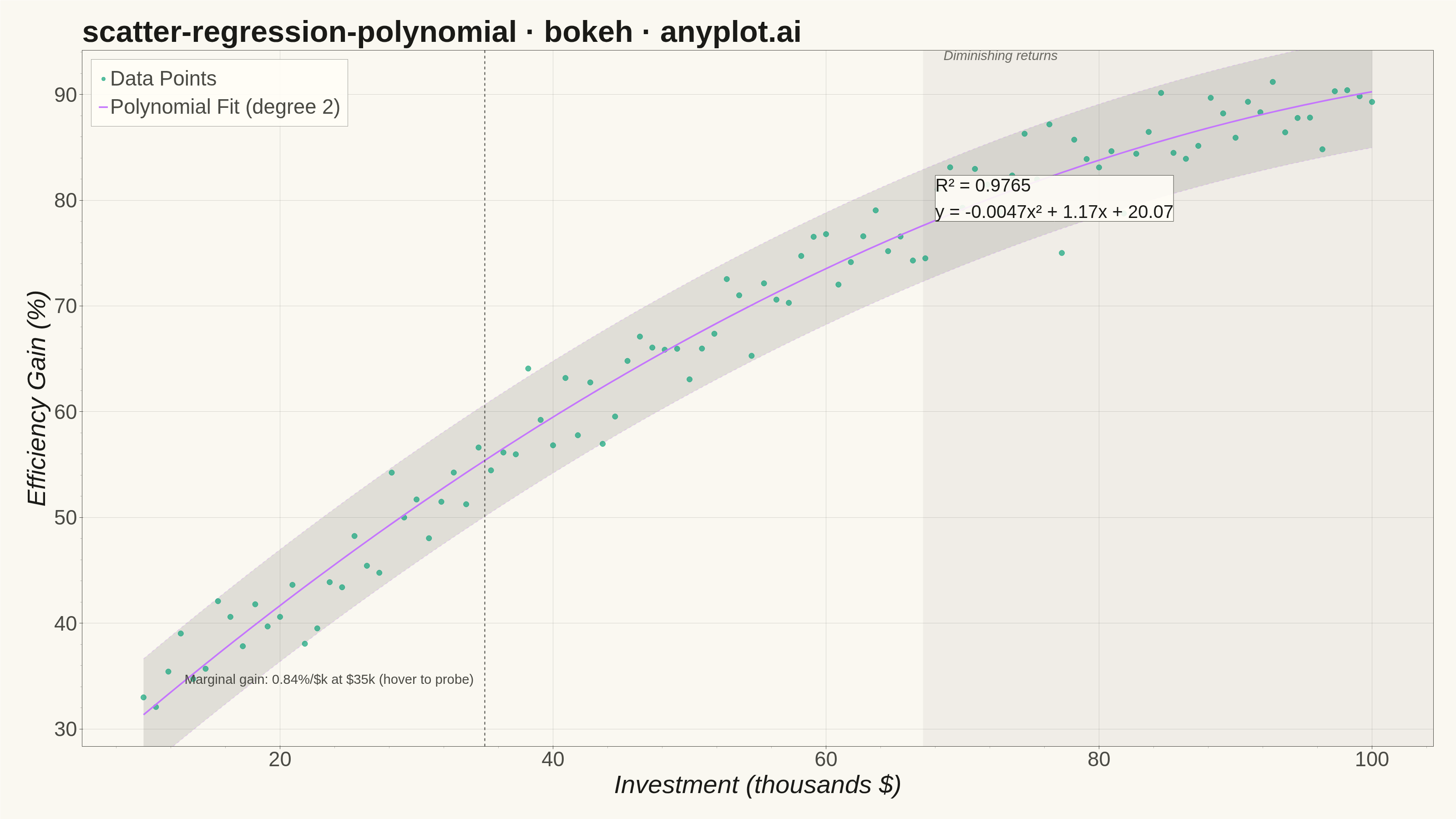
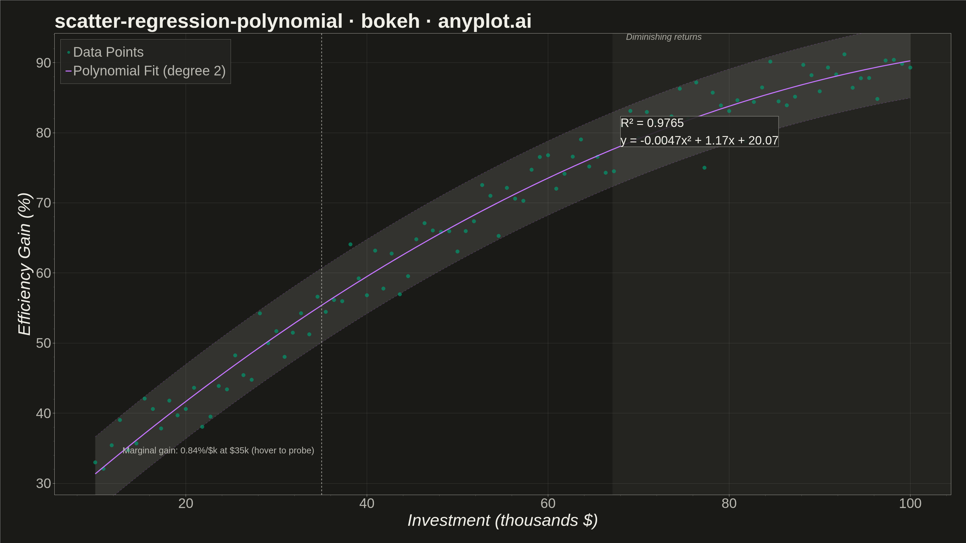
Scatter Plot with Polynomial Regression — Bokeh

A scatter plot displaying the relationship between two numeric variables with a fitted polynomial regression curve (degree 2-4). This visualization extends beyond linear regression to capture non-linear relationships in data, making it ideal for modeling curved trends, parabolic patterns, and complex data relationships where a straight line would not adequately represent the underlying pattern.

Scatter Plot with Polynomial Regression rendered with Bokeh

Python source (Bokeh)

""" anyplot.ai
scatter-regression-polynomial: Scatter Plot with Polynomial Regression
Library: bokeh 3.9.0 | Python 3.13.13
Quality: 88/100 | Updated: 2026-05-07
"""

import os
import time
from pathlib import Path

import numpy as np
from bokeh.io import output_file, save
from bokeh.models import ColumnDataSource, HoverTool, Label
from bokeh.plotting import figure
from selenium import webdriver
from selenium.webdriver.chrome.options import Options


# Theme tokens
THEME = os.getenv("ANYPLOT_THEME", "light")
PAGE_BG = "#FAF8F1" if THEME == "light" else "#1A1A17"
ELEVATED_BG = "#FFFDF6" if THEME == "light" else "#242420"
INK = "#1A1A17" if THEME == "light" else "#F0EFE8"
INK_SOFT = "#4A4A44" if THEME == "light" else "#B8B7B0"

# Okabe-Ito palette
BRAND = "#009E73"  # First series - always green
ACCENT = "#C475FD"  # Second series - vermillion for contrast

# Data - Manufacturing efficiency curve (diminishing returns pattern)
np.random.seed(42)
n_points = 100

# Investment amount (thousands of dollars)
x = np.linspace(10, 100, n_points)
# Efficiency gains follow a quadratic pattern with diminishing returns
# True relationship: y = -0.005x^2 + 1.2x + 20 + noise
y = -0.005 * x**2 + 1.2 * x + 20 + np.random.normal(0, 3, n_points)

# Polynomial regression (degree 2 - quadratic)
coeffs = np.polyfit(x, y, 2)
poly = np.poly1d(coeffs)

# Calculate R-squared
y_pred = poly(x)
ss_res = np.sum((y - y_pred) ** 2)
ss_tot = np.sum((y - np.mean(y)) ** 2)
r_squared = 1 - (ss_res / ss_tot)

# Create smooth curve for regression line
x_smooth = np.linspace(x.min(), x.max(), 200)
y_smooth = poly(x_smooth)

# Format polynomial equation
a, b, c = coeffs
equation = f"y = {a:.4f}x² + {b:.2f}x + {c:.2f}"

# Create data sources
scatter_source = ColumnDataSource(data={"x": x, "y": y})
line_source = ColumnDataSource(data={"x": x_smooth, "y": y_smooth})

# Create figure (4800 x 2700 px)
p = figure(
    width=4800,
    height=2700,
    title="scatter-regression-polynomial · bokeh · anyplot.ai",
    x_axis_label="Investment (thousands $)",
    y_axis_label="Efficiency Gain (%)",
)

# Plot scatter points
p.scatter(x="x", y="y", source=scatter_source, size=18, color=BRAND, alpha=0.65, legend_label="Data Points")

# Plot polynomial regression curve
p.line(x="x", y="y", source=line_source, line_width=5, color=ACCENT, legend_label="Polynomial Fit (degree 2)")

# Add HoverTool for interactivity
hover = HoverTool(tooltips=[("Investment", "@x{0.0}"), ("Efficiency", "@y{0.0}")])
p.add_tools(hover)

# Add R² and equation annotation
annotation_text = f"R² = {r_squared:.4f}\n{equation}"
annotation = Label(
    x=70,
    y=75,
    text=annotation_text,
    text_font_size="24pt",
    text_color=INK,
    background_fill_color=ELEVATED_BG,
    background_fill_alpha=0.9,
    border_line_color=INK_SOFT,
)
p.add_layout(annotation)

# Styling - Text sizes for 4800x2700 canvas
p.title.text_font_size = "28pt"
p.title.text_color = INK
p.xaxis.axis_label_text_font_size = "22pt"
p.yaxis.axis_label_text_font_size = "22pt"
p.xaxis.axis_label_text_color = INK
p.yaxis.axis_label_text_color = INK
p.xaxis.major_label_text_font_size = "18pt"
p.yaxis.major_label_text_font_size = "18pt"
p.xaxis.major_label_text_color = INK_SOFT
p.yaxis.major_label_text_color = INK_SOFT

# Grid styling
p.xgrid.grid_line_color = INK
p.ygrid.grid_line_color = INK
p.xgrid.grid_line_alpha = 0.10
p.ygrid.grid_line_alpha = 0.10

# Legend styling - top left placement for better visibility
p.legend.location = "top_left"
p.legend.label_text_font_size = "18pt"
p.legend.label_text_color = INK_SOFT
p.legend.background_fill_color = ELEVATED_BG
p.legend.background_fill_alpha = 0.9
p.legend.border_line_color = INK_SOFT

# Background and outline
p.background_fill_color = PAGE_BG
p.border_fill_color = PAGE_BG
p.outline_line_color = INK_SOFT

# Save as HTML
output_file(f"plot-{THEME}.html")
save(p)

# Screenshot with headless Chrome using Selenium
W, H = 4800, 2700
opts = Options()
for arg in (
    "--headless=new",
    "--no-sandbox",
    "--disable-dev-shm-usage",
    "--disable-gpu",
    f"--window-size={W},{H}",
    "--hide-scrollbars",
):
    opts.add_argument(arg)
driver = webdriver.Chrome(options=opts)
driver.set_window_size(W, H)
driver.get(f"file://{Path(f'plot-{THEME}.html').resolve()}")
time.sleep(3)
driver.save_screenshot(f"plot-{THEME}.png")
driver.quit()

Part of Scatter Plot with Polynomial Regression on anyplot.ai.

Scatter Plot with Polynomial Regression — Bokeh

Python source (Bokeh)

Other implementations