The same plot in 14 other libraries — Python: Altair, Bokeh, lets-plot, Matplotlib, Plotly, plotnine, Pygal, Seaborn; R: ggplot2; JavaScript: Chart.js, D3.js, Apache ECharts, Highcharts, MUI X Charts. Compare all 15 side by side: Scatter Plot with Polynomial Regression in Python, R, Julia and JavaScript.
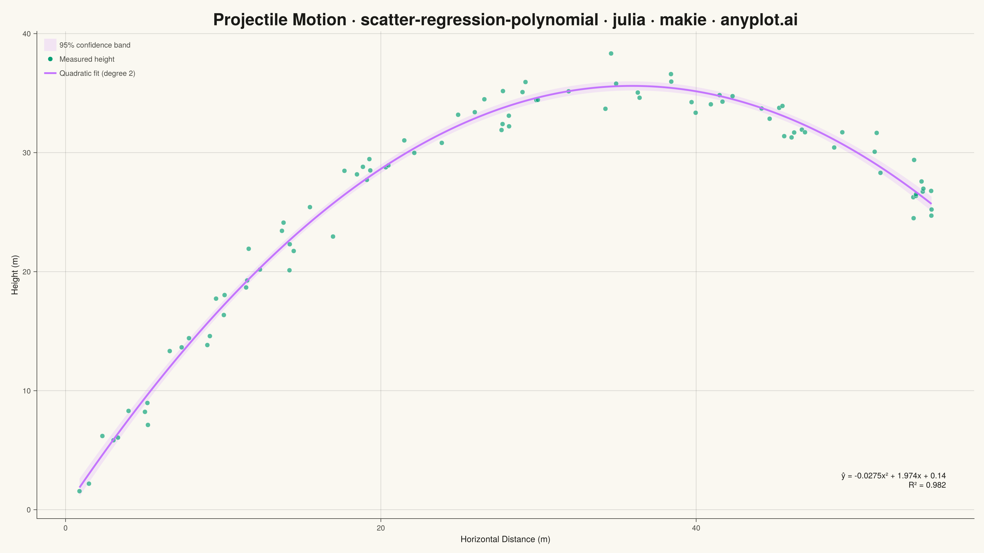
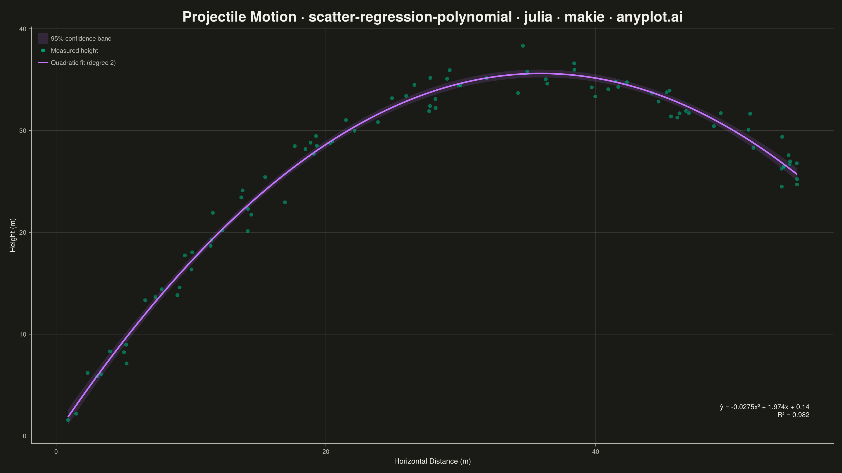
A scatter plot displaying the relationship between two numeric variables with a fitted polynomial regression curve (degree 2-4). This visualization extends beyond linear regression to capture non-linear relationships in data, making it ideal for modeling curved trends, parabolic patterns, and complex data relationships where a straight line would not adequately represent the underlying pattern.
# anyplot.ai
# scatter-regression-polynomial: Scatter Plot with Polynomial Regression
# Library: makie 0.21.9 | Julia 1.11.9
# Quality: 90/100 | Created: 2026-08-11

using CairoMakie
using Colors
using Random
using Statistics

Random.seed!(42)

# --- Theme tokens -------------------------------------------------------------
const THEME    = get(ENV, "ANYPLOT_THEME", "light")
const PAGE_BG  = THEME == "light" ? colorant"#FAF8F1" : colorant"#1A1A17"
const INK      = THEME == "light" ? colorant"#1A1A17" : colorant"#F0EFE8"
const INK_SOFT = THEME == "light" ? colorant"#4A4A44" : colorant"#B8B7B0"
const IMPRINT_PALETTE = [
    colorant"#009E73", colorant"#C475FD", colorant"#4467A3", colorant"#BD8233",
    colorant"#AE3030", colorant"#2ABCCD", colorant"#954477", colorant"#99B314",
]
const BRAND = IMPRINT_PALETTE[1]
const FIT_COLOR = IMPRINT_PALETTE[2]

# --- Data: cannon-launch trajectory measurements -------------------------------
n_shots = 90
horizontal_distance_m = sort(rand(n_shots) .* 55.0)
true_a, true_b, true_c = -0.028, 2.0, 0.0
height_true_m = true_a .* horizontal_distance_m .^ 2 .+ true_b .* horizontal_distance_m .+ true_c
height_m = height_true_m .+ randn(n_shots) .* 1.3

# --- Quadratic least-squares fit (Vandermonde design, degree 2) ----------------
degree = 2
X = hcat(ones(n_shots), horizontal_distance_m, horizontal_distance_m .^ 2)
coeffs = X \ height_m
fitted_m = X * coeffs
residuals = height_m .- fitted_m
sse = sum(residuals .^ 2)
sst = sum((height_m .- mean(height_m)) .^ 2)
r_squared = 1 - sse / sst
mse = sse / (n_shots - (degree + 1))
xtx = X' * X

x_grid = range(minimum(horizontal_distance_m), maximum(horizontal_distance_m), length = 200)
X_grid = hcat(ones(length(x_grid)), collect(x_grid), collect(x_grid) .^ 2)
y_grid = X_grid * coeffs
se_grid = [sqrt(mse * (X_grid[i, :]' * (xtx \ X_grid[i, :]))) for i in 1:size(X_grid, 1)]
y_lower = y_grid .- 1.96 .* se_grid
y_upper = y_grid .+ 1.96 .* se_grid

# --- Equation + goodness-of-fit annotation text --------------------------------
b_sign = coeffs[2] >= 0 ? "+" : "-"
c_sign = coeffs[1] >= 0 ? "+" : "-"
eqn_text = "ŷ = $(round(coeffs[3], digits=4))x² $(b_sign) $(abs(round(coeffs[2], digits=3)))x $(c_sign) $(abs(round(coeffs[1], digits=2)))\nR² = $(round(r_squared, digits=3))"

# --- Plot -----------------------------------------------------------------------
title_str = "Projectile Motion · scatter-regression-polynomial · julia · makie · anyplot.ai"
title_fontsize = max(18, round(Int, 32 * 67 / length(title_str)))

fig = Figure(
    resolution = (1600, 900),
    fontsize = 14,
    backgroundcolor = PAGE_BG,
)

ax = Axis(
    fig[1, 1];
    title = title_str,
    titlesize = title_fontsize,
    titlecolor = INK,
    xlabel = "Horizontal Distance (m)",
    ylabel = "Height (m)",
    xlabelsize = 14,
    ylabelsize = 14,
    xlabelcolor = INK,
    ylabelcolor = INK,
    xticklabelsize = 12,
    yticklabelsize = 12,
    xticklabelcolor = INK_SOFT,
    yticklabelcolor = INK_SOFT,
    xtickcolor = INK_SOFT,
    ytickcolor = INK_SOFT,
    backgroundcolor = PAGE_BG,
    topspinevisible = false,
    rightspinevisible = false,
    leftspinecolor = INK_SOFT,
    bottomspinecolor = INK_SOFT,
    xgridcolor = RGBAf(INK.r, INK.g, INK.b, 0.15),
    ygridcolor = RGBAf(INK.r, INK.g, INK.b, 0.15),
    xminorgridvisible = false,
    yminorgridvisible = false,
)

band!(ax, x_grid, y_lower, y_upper;
      color = RGBAf(FIT_COLOR.r, FIT_COLOR.g, FIT_COLOR.b, 0.15),
      label = "95% confidence band")
scatter!(ax, horizontal_distance_m, height_m;
         color = BRAND, alpha = 0.65, markersize = 11,
         strokecolor = PAGE_BG, strokewidth = 0.5,
         label = "Measured height")
lines!(ax, x_grid, y_grid; color = FIT_COLOR, linewidth = 3.0, label = "Quadratic fit (degree 2)")

text!(ax, 0.97, 0.06, text = eqn_text, space = :relative,
      align = (:right, :bottom), fontsize = 13, color = INK)

axislegend(ax, position = :lt, framevisible = false, labelsize = 12, labelcolor = INK_SOFT)

# --- Save -------------------------------------------------------------------
save("plot-$(THEME).png", fig; px_per_unit = 2)
Runnable source as JSON, for any HTTP client: https://api.anyplot.ai/specs/scatter-regression-polynomial/makie/code. Any spec id and library id listed in llms-full.txt fit the same URL shape; every URL below is complete and callable.
{
  "spec_id": "scatter-regression-polynomial",
  "language": "julia",
  "library": "makie",
  "page": "https://anyplot.ai/scatter-regression-polynomial/julia/makie",
  "hub": "https://anyplot.ai/scatter-regression-polynomial",
  "code_json": "https://api.anyplot.ai/specs/scatter-regression-polynomial/makie/code",
  "spec_json": "https://api.anyplot.ai/specs/scatter-regression-polynomial",
  "render_light_png": "https://storage.googleapis.com/anyplot-images/plots/scatter-regression-polynomial/julia/makie/plot-light.png",
  "render_dark_png": "https://storage.googleapis.com/anyplot-images/plots/scatter-regression-polynomial/julia/makie/plot-dark.png",
  "quality_score": 90.0,
  "license": "MIT",
  "guide": "https://anyplot.ai/llms.txt"
}
Part of Scatter Plot with Polynomial Regression on anyplot.ai.