The same plot in 14 other libraries — JavaScript: Chart.js, D3.js, Apache ECharts, Highcharts; Python: Altair, Bokeh, lets-plot, Matplotlib, Plotly, plotnine, Pygal, Seaborn; R: ggplot2; Julia: Makie.jl. Compare all 15 side by side: Scatter Plot with Polynomial Regression in Python, R, Julia and JavaScript.
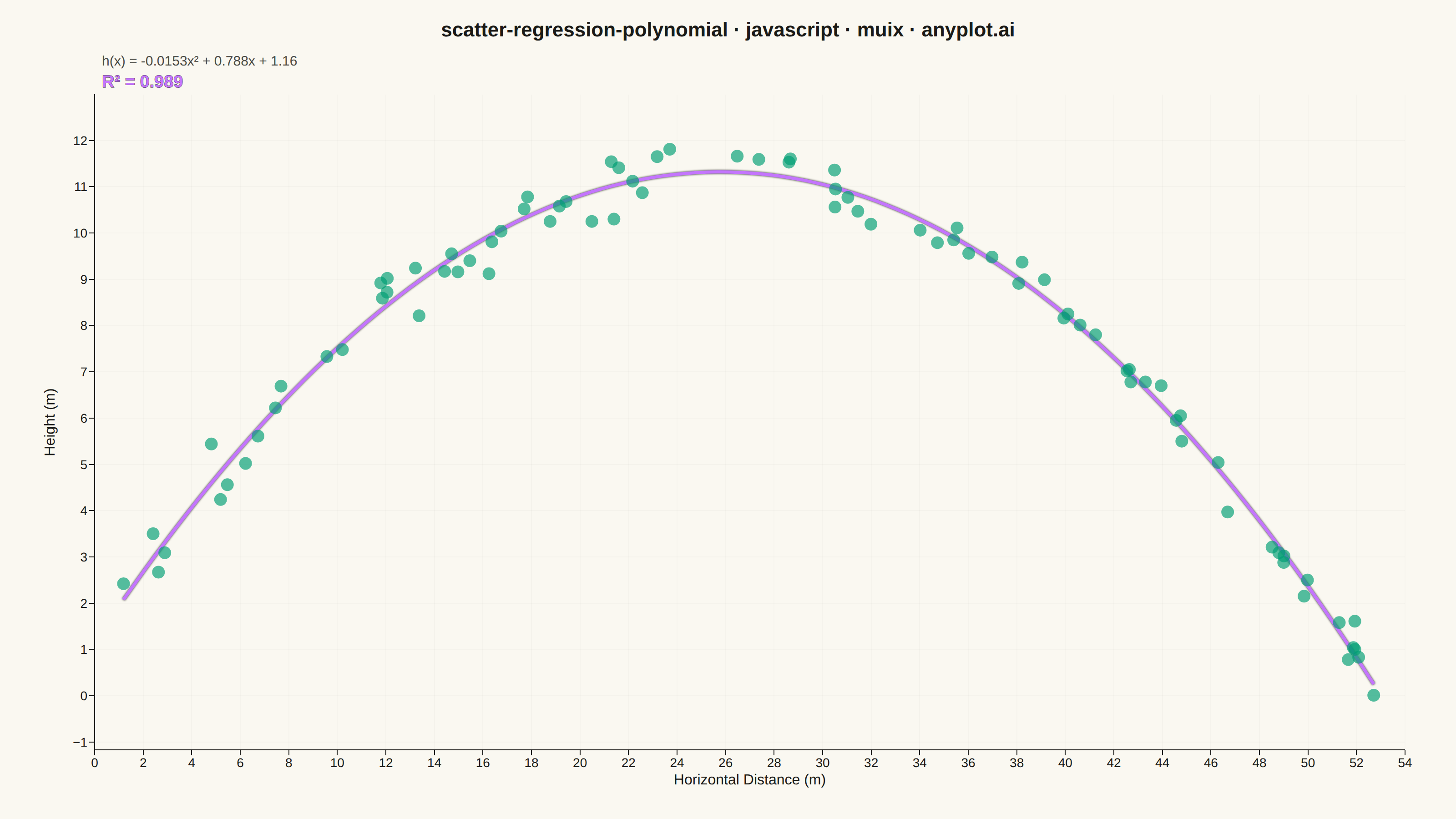
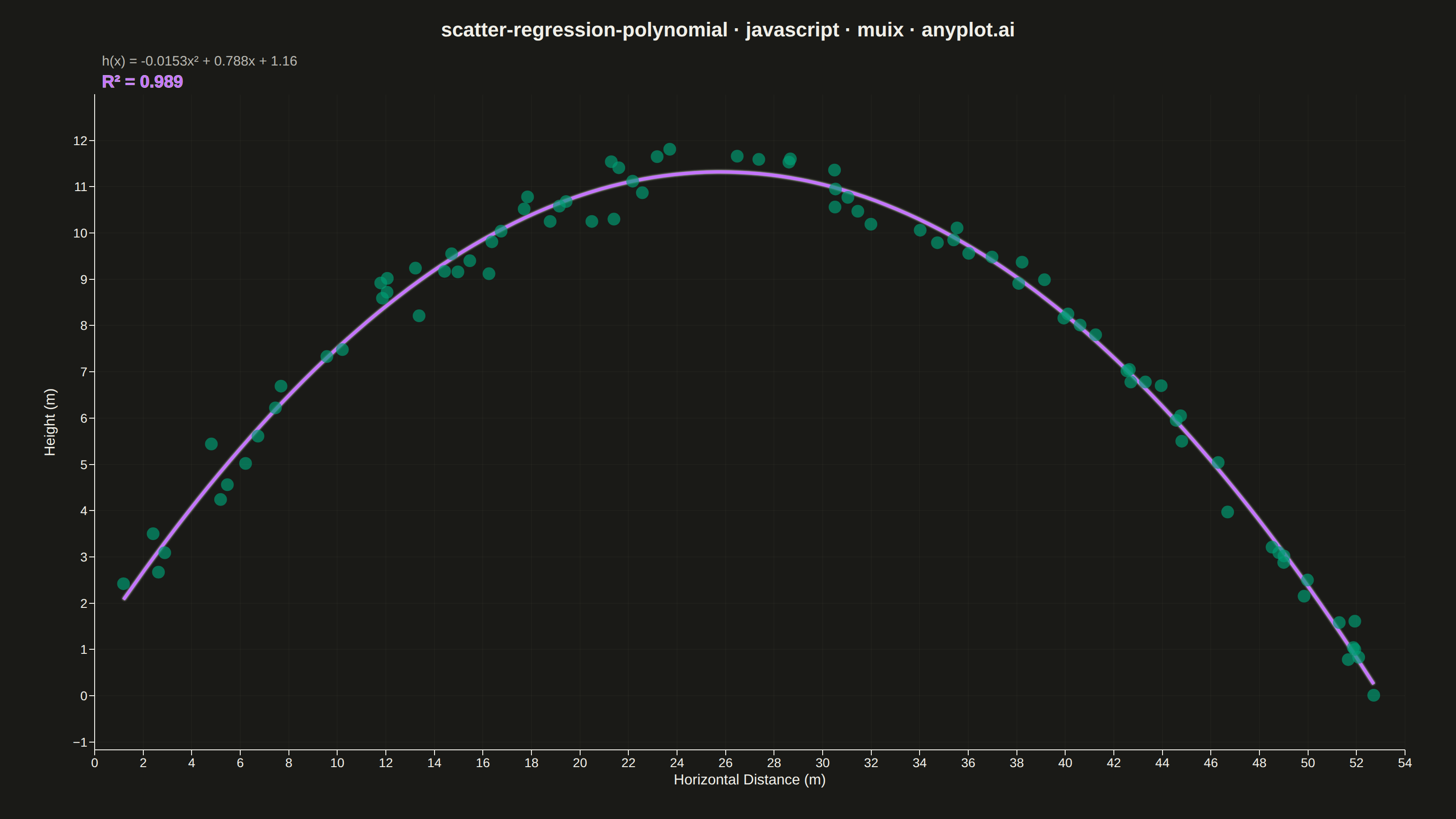
A scatter plot displaying the relationship between two numeric variables with a fitted polynomial regression curve (degree 2-4). This visualization extends beyond linear regression to capture non-linear relationships in data, making it ideal for modeling curved trends, parabolic patterns, and complex data relationships where a straight line would not adequately represent the underlying pattern.
// anyplot.ai
// scatter-regression-polynomial: Scatter Plot with Polynomial Regression
// Library: muix 7.29.1 | JavaScript 22.23.1
// Quality: 91/100 | Created: 2026-08-11
import { ChartContainer } from "@mui/x-charts/ChartContainer";
import { ScatterPlot } from "@mui/x-charts/ScatterChart";
import { LinePlot } from "@mui/x-charts/LineChart";
import { ChartsXAxis } from "@mui/x-charts/ChartsXAxis";
import { ChartsYAxis } from "@mui/x-charts/ChartsYAxis";
import { ChartsGrid } from "@mui/x-charts/ChartsGrid";

const t = window.ANYPLOT_TOKENS;

// --- Deterministic PRNG (LCG) + Box-Muller for reproducible normal noise ----
function makeLcg(seed: number) {
  let state = seed;
  return function next() {
    state = (state * 1664525 + 1013904223) % 4294967296;
    return state / 4294967296;
  };
}
function randNormal(rand: () => number) {
  const u1 = Math.max(rand(), 1e-9);
  const u2 = rand();
  return Math.sqrt(-2 * Math.log(u1)) * Math.cos(2 * Math.PI * u2);
}

// --- Least-squares polynomial fit via normal equations (Gauss-Jordan) -------
function polyFit(xs: number[], ys: number[], degree: number) {
  const size = degree + 1;
  const ata: number[][] = Array.from({ length: size }, () => new Array(size).fill(0));
  const aty: number[] = new Array(size).fill(0);
  for (let i = 0; i < xs.length; i += 1) {
    const powers: number[] = new Array(size);
    let p = 1;
    for (let k = 0; k < size; k += 1) {
      powers[k] = p;
      p *= xs[i];
    }
    for (let r = 0; r < size; r += 1) {
      aty[r] += powers[r] * ys[i];
      for (let c = 0; c < size; c += 1) ata[r][c] += powers[r] * powers[c];
    }
  }
  // Gauss-Jordan elimination on the augmented [ata | aty] system, in place.
  const augmented = ata.map((row, i) => [...row, aty[i]]);
  for (let col = 0; col < size; col += 1) {
    let pivotRow = col;
    for (let row = col + 1; row < size; row += 1) {
      if (Math.abs(augmented[row][col]) > Math.abs(augmented[pivotRow][col])) {
        pivotRow = row;
      }
    }
    [augmented[col], augmented[pivotRow]] = [augmented[pivotRow], augmented[col]];
    const pivot = augmented[col][col];
    for (let c = col; c <= size; c += 1) augmented[col][c] /= pivot;
    for (let row = 0; row < size; row += 1) {
      if (row === col) continue;
      const factor = augmented[row][col];
      for (let c = col; c <= size; c += 1) augmented[row][c] -= factor * augmented[col][c];
    }
  }
  return augmented.map((row) => row[size]); // ascending powers: [c0, c1, c2, ...]
}

function evalPoly(coeffs: number[], x: number) {
  let y = 0;
  let p = 1;
  for (let i = 0; i < coeffs.length; i += 1) {
    y += coeffs[i] * p;
    p *= x;
  }
  return y;
}

// --- Data: projectile trajectory — horizontal distance vs. height -----------
// Tracked ball flight: h(x) = -g/(2*v0x^2)*x^2 + (v0y/v0x)*x + h0, plus sensor noise.
const rand = makeLcg(42);
const V0X = 18; // m/s horizontal velocity
const V0Y = 14; // m/s vertical velocity
const H0 = 1.3; // m release height
const G = 9.81; // m/s^2
const trueA = -G / (2 * V0X ** 2);
const trueB = V0Y / V0X;
const trueC = H0;
const flightRange = (-trueB - Math.sqrt(trueB ** 2 - 4 * trueA * trueC)) / (2 * trueA);

const POINT_COUNT = 85;
const distance: number[] = [];
const height: number[] = [];
for (let i = 0; i < POINT_COUNT; i += 1) {
  const x = rand() * flightRange;
  const trueY = trueA * x ** 2 + trueB * x + trueC;
  const measured = Math.max(trueY + randNormal(rand) * 0.4, 0);
  distance.push(Number(x.toFixed(2)));
  height.push(Number(measured.toFixed(2)));
}

// --- Quadratic regression + goodness of fit ----------------------------------
const coeffs = polyFit(distance, height, 2);
const n = height.length;
const yMean = height.reduce((sum, y) => sum + y, 0) / n;
let ssRes = 0;
let ssTot = 0;
for (let i = 0; i < n; i += 1) {
  const fitted = evalPoly(coeffs, distance[i]);
  ssRes += (height[i] - fitted) ** 2;
  ssTot += (height[i] - yMean) ** 2;
}
const rSquared = 1 - ssRes / ssTot;

const CURVE_POINTS = 60;
const xMin = Math.min(...distance);
const xMax = Math.max(...distance);
const curveX = Array.from(
  { length: CURVE_POINTS },
  (_, i) => xMin + ((xMax - xMin) * i) / (CURVE_POINTS - 1),
);
const curveY = curveX.map((x) => evalPoly(coeffs, x));

const scatterData = distance.map((x, i) => ({ x, y: height[i], id: `pt-${i}` }));

const yAllValues = [...height, ...curveY];
const yPad = (Math.max(...yAllValues) - Math.min(...yAllValues)) * 0.1;
const yDomainMin = Math.min(0, Math.min(...yAllValues) - yPad);
const yDomainMax = Math.max(...yAllValues) + yPad;

const regressionColor = t.palette[1]; // lavender — canonical Imprint position 2

const linearTerm = `${coeffs[1] >= 0 ? "+" : "-"} ${Math.abs(coeffs[1]).toFixed(3)}`;
const constantTerm = `${coeffs[0] >= 0 ? "+" : "-"} ${Math.abs(coeffs[0]).toFixed(2)}`;
const equationLabel = `h(x) = ${coeffs[2].toFixed(4)}x² ${linearTerm}x ${constantTerm}`;
const fitLabel = `R² = ${rSquared.toFixed(3)}`;

const title = "scatter-regression-polynomial · javascript · muix · anyplot.ai";

// --- Chart (default-exported component — the harness mounts it) ------------
export default function Chart() {
  const { width, height: chartHeight } = window.ANYPLOT_SIZE;

  return (
    <ChartContainer
      width={width}
      height={chartHeight}
      margin={{ top: 104, right: 56, bottom: 76, left: 104 }}
      series={[
        {
          type: "scatter",
          id: "observations",
          data: scatterData,
          markerSize: 7,
          color: `${t.palette[0]}aa`,
        },
        {
          type: "line",
          id: "regression",
          data: curveY,
          curve: "natural",
          color: regressionColor,
          showMark: false,
          disableHighlight: true,
        },
      ]}
      xAxis={[
        {
          data: curveX,
          scaleType: "linear",
          label: "Horizontal Distance (m)",
          tickLabelStyle: { fontSize: 14 },
          labelStyle: { fontSize: 16 },
        },
      ]}
      yAxis={[
        {
          scaleType: "linear",
          min: yDomainMin,
          max: yDomainMax,
          label: "Height (m)",
          tickFontSize: 28,
          tickLabelStyle: { fontSize: 14 },
          labelStyle: { fontSize: 16 },
        },
      ]}
      skipAnimation
    >
      <ChartsGrid
        vertical
        horizontal
        sx={{ "& line": { stroke: t.grid, strokeOpacity: 0.15 } }}
      />
      <LinePlot
        skipAnimation
        slotProps={{
          line: {
            style: { strokeWidth: 3.5, filter: `drop-shadow(0 0 1px ${t.ink})` },
          },
        }}
      />
      <ScatterPlot />
      <ChartsXAxis />
      <ChartsYAxis />
      <text
        x={width / 2}
        y={40}
        textAnchor="middle"
        fontSize={22}
        fontWeight={600}
        fill={t.ink}
      >
        {title}
      </text>
      <text x={112} y={72} fontSize={15} fill={t.inkSoft}>
        {equationLabel}
      </text>
      <text
        x={112}
        y={96}
        fontSize={19}
        fontWeight={700}
        fill={regressionColor}
        stroke={t.ink}
        strokeWidth={0.5}
        paintOrder="stroke"
      >
        {fitLabel}
      </text>
    </ChartContainer>
  );
}
Runnable source as JSON, for any HTTP client: https://api.anyplot.ai/specs/scatter-regression-polynomial/muix/code. Any spec id and library id listed in llms-full.txt fit the same URL shape; every URL below is complete and callable.
{
  "spec_id": "scatter-regression-polynomial",
  "language": "javascript",
  "library": "muix",
  "page": "https://anyplot.ai/scatter-regression-polynomial/javascript/muix",
  "hub": "https://anyplot.ai/scatter-regression-polynomial",
  "code_json": "https://api.anyplot.ai/specs/scatter-regression-polynomial/muix/code",
  "spec_json": "https://api.anyplot.ai/specs/scatter-regression-polynomial",
  "render_light_png": "https://storage.googleapis.com/anyplot-images/plots/scatter-regression-polynomial/javascript/muix/plot-light.png",
  "render_dark_png": "https://storage.googleapis.com/anyplot-images/plots/scatter-regression-polynomial/javascript/muix/plot-dark.png",
  "interactive_light_html": "https://storage.googleapis.com/anyplot-images/plots/scatter-regression-polynomial/javascript/muix/plot-light.html",
  "interactive_dark_html": "https://storage.googleapis.com/anyplot-images/plots/scatter-regression-polynomial/javascript/muix/plot-dark.html",
  "quality_score": 91.0,
  "license": "MIT",
  "guide": "https://anyplot.ai/llms.txt"
}
Part of Scatter Plot with Polynomial Regression on anyplot.ai.