The same plot in 14 other libraries — Python: Altair, Bokeh, lets-plot, Matplotlib, Plotly, plotnine, Pygal, Seaborn; R: ggplot2; JavaScript: Chart.js, D3.js, Apache ECharts, Highcharts, MUI X Charts. Compare all 15 side by side: SHAP Summary Plot in Python, R, Julia and JavaScript.
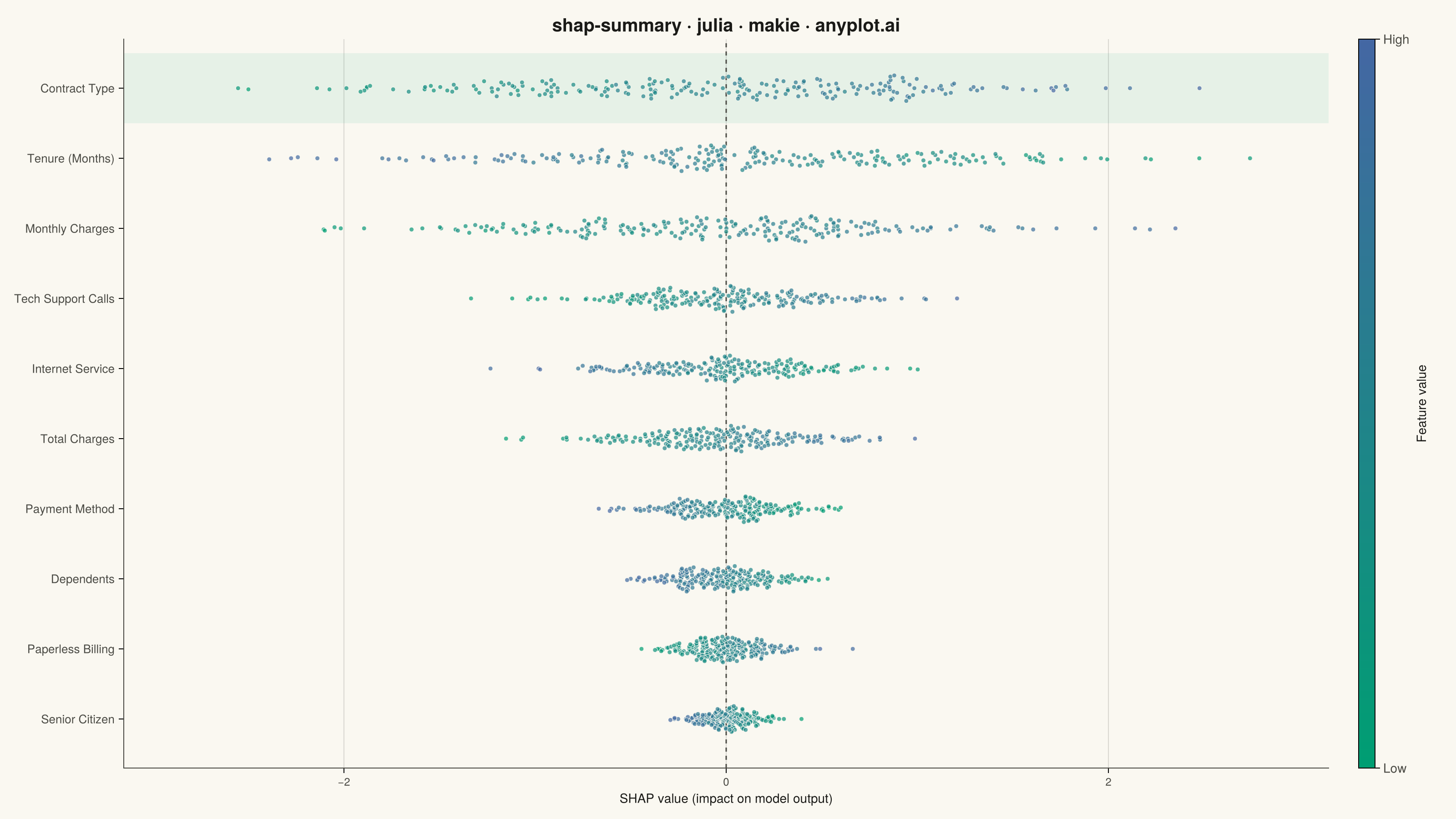
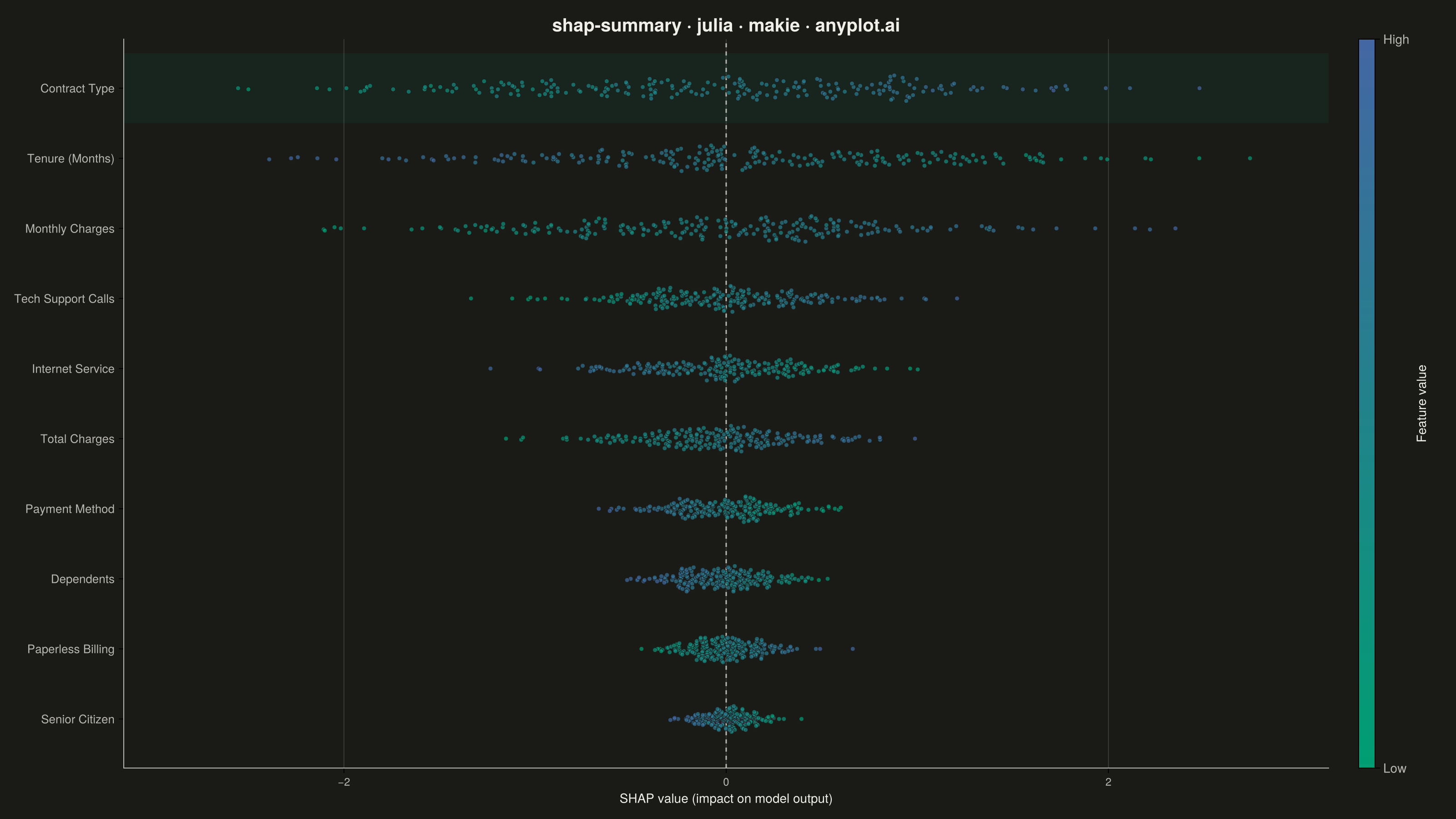
A SHAP (SHapley Additive exPlanations) summary plot displaying the distribution of SHAP values for each feature, ordered by mean absolute SHAP value (importance). Each dot represents a sample, positioned horizontally by its SHAP value and colored by the feature's value (typically low=blue to high=red). This visualization is essential for machine learning interpretability, showing both feature importance and the direction and magnitude of feature effects on model predictions.
# anyplot.ai
# shap-summary: SHAP Summary Plot
# Library: makie 0.21.9 | Julia 1.11.9
# Quality: 92/100 | Created: 2026-09-09

using CairoMakie
using Makie
using Colors
using Random
using Statistics

Random.seed!(42)

# --- Theme tokens ------------------------------------------------------------
THEME    = get(ENV, "ANYPLOT_THEME", "light")
PAGE_BG  = THEME == "light" ? colorant"#FAF8F1" : colorant"#1A1A17"
INK      = THEME == "light" ? colorant"#1A1A17" : colorant"#F0EFE8"
INK_SOFT = THEME == "light" ? colorant"#4A4A44" : colorant"#B8B7B0"

# Continuous feature-value scale — Imprint sequential (green -> blue)
IMPRINT_SEQ = cgrad([colorant"#009E73", colorant"#4467A3"])

# --- Data ---------------------------------------------------------------------
# Synthetic SHAP output for a customer-churn classifier (TreeExplainer-style).
feature_names_raw = [
    "Contract Type", "Tenure (Months)", "Monthly Charges", "Tech Support Calls",
    "Internet Service", "Total Charges", "Payment Method", "Dependents",
    "Paperless Billing", "Senior Citizen",
]
n_features = length(feature_names_raw)
n_samples  = 220

# Per-feature effect scale (drives mean |SHAP|) and sign of the value-effect
# correlation (a high feature value can push the prediction up OR down).
effect_scale = [0.95, 0.85, 0.78, 0.42, 0.38, 0.34, 0.24, 0.20, 0.16, 0.12]
direction    = [1, -1, 1, 1, -1, 1, -1, -1, 1, -1]

feature_values_raw = randn(n_samples, n_features)
shap_values_raw = similar(feature_values_raw)
for j in 1:n_features
    signal = direction[j] .* feature_values_raw[:, j] .* effect_scale[j]
    noise = randn(n_samples) .* effect_scale[j] .* 0.35
    shap_values_raw[:, j] = signal .+ noise
end

# Sort features by mean absolute SHAP value — most important at the top.
mean_abs_shap = vec(mean(abs.(shap_values_raw), dims = 1))
order = sortperm(mean_abs_shap, rev = true)

feature_names = feature_names_raw[order]
feature_values = feature_values_raw[:, order]
shap_values = shap_values_raw[:, order]

# Per-feature min-max scaling of the raw feature value, used for point color.
color_values = similar(feature_values)
for j in 1:n_features
    col = feature_values[:, j]
    lo, hi = extrema(col)
    color_values[:, j] = (col .- lo) ./ (hi - lo)
end

# Beeswarm-style vertical jitter: bin each feature's SHAP values, then stack
# same-bin points alternately above/below the row center to avoid overlap.
n_bins = 24
jitter_width = 0.38
row_offsets = similar(shap_values)
for j in 1:n_features
    values = shap_values[:, j]
    lo, hi = extrema(values)
    edges = range(lo, hi, length = n_bins + 1)
    bin_id = Vector{Int}(undef, n_samples)
    for i in 1:n_samples
        bin_id[i] = clamp(searchsortedlast(edges, values[i]), 1, n_bins)
    end
    counts = zeros(Int, n_bins)
    offsets = zeros(Float64, n_samples)
    for i in 1:n_samples
        b = bin_id[i]
        k = counts[b]
        sgn = isodd(k) ? -1.0 : 1.0
        offsets[i] = sgn * ceil(k / 2)
        counts[b] += 1
    end
    row_offsets[:, j] = offsets ./ max(maximum(counts), 1) .* jitter_width
end

# Flatten into plotting vectors (column-major: feature 1's samples first).
xs = vec(shap_values)
colors = vec(color_values)
ys = Vector{Float64}(undef, n_samples * n_features)
for j in 1:n_features
    y_base = n_features - j + 1  # rank 1 (most important) sits at the top
    rng = ((j - 1) * n_samples + 1):(j * n_samples)
    ys[rng] = fill(Float64(y_base), n_samples) .+ row_offsets[:, j]
end

max_abs_shap = maximum(abs.(xs)) * 1.15

# --- Plot ----------------------------------------------------------------------
fig = Figure(
    resolution = (1600, 900),
    fontsize = 14,
    backgroundcolor = PAGE_BG,
)

ax = Axis(
    fig[1, 1];
    title = "shap-summary · julia · makie · anyplot.ai",
    titlesize = 20,
    titlecolor = INK,
    xlabel = "SHAP value (impact on model output)",
    xlabelsize = 14,
    xlabelcolor = INK,
    xticklabelsize = 12,
    xticklabelcolor = INK_SOFT,
    yticklabelsize = 13,
    yticklabelcolor = INK_SOFT,
    backgroundcolor = PAGE_BG,
    topspinevisible = false,
    rightspinevisible = false,
    leftspinecolor = INK_SOFT,
    bottomspinecolor = INK_SOFT,
    xgridcolor = RGBAf(INK.r, INK.g, INK.b, 0.15),
    ygridvisible = false,
    yticks = (1:n_features, reverse(feature_names)),
)
xlims!(ax, -max_abs_shap, max_abs_shap)
ylims!(ax, 0.3, n_features + 0.7)

# Subtle accent band behind the top (most important) feature row, drawn
# before the scatter so it sits underneath the data points.
top_row_y = Float64(n_features)
hspan!(
    ax, top_row_y - 0.5, top_row_y + 0.5;
    color = RGBAf(colorant"#009E73".r, colorant"#009E73".g, colorant"#009E73".b, 0.08),
)

vlines!(ax, 0; color = INK_SOFT, linewidth = 1.5, linestyle = :dash)

scatter!(
    ax, xs, ys;
    color = colors,
    colormap = IMPRINT_SEQ,
    colorrange = (0, 1),
    markersize = 7,
    strokewidth = 0.5,
    strokecolor = PAGE_BG,
    alpha = 0.7,
)

Colorbar(
    fig[1, 2];
    colormap = IMPRINT_SEQ,
    limits = (0, 1),
    label = "Feature value",
    labelcolor = INK,
    ticks = ([0, 1], ["Low", "High"]),
    ticklabelcolor = INK_SOFT,
    width = 18,
)
colsize!(fig.layout, 2, Relative(0.035))

# --- Save ------------------------------------------------------------------
save("plot-$(THEME).png", fig; px_per_unit = 2)
Runnable source as JSON, for any HTTP client: https://api.anyplot.ai/specs/shap-summary/makie/code. Any spec id and library id listed in llms-full.txt fit the same URL shape; every URL below is complete and callable.
{
  "spec_id": "shap-summary",
  "language": "julia",
  "library": "makie",
  "page": "https://anyplot.ai/shap-summary/julia/makie",
  "hub": "https://anyplot.ai/shap-summary",
  "code_json": "https://api.anyplot.ai/specs/shap-summary/makie/code",
  "spec_json": "https://api.anyplot.ai/specs/shap-summary",
  "render_light_png": "https://storage.googleapis.com/anyplot-images/plots/shap-summary/julia/makie/plot-light.png",
  "render_dark_png": "https://storage.googleapis.com/anyplot-images/plots/shap-summary/julia/makie/plot-dark.png",
  "quality_score": 92.0,
  "license": "MIT",
  "guide": "https://anyplot.ai/llms.txt"
}
Part of SHAP Summary Plot on anyplot.ai.