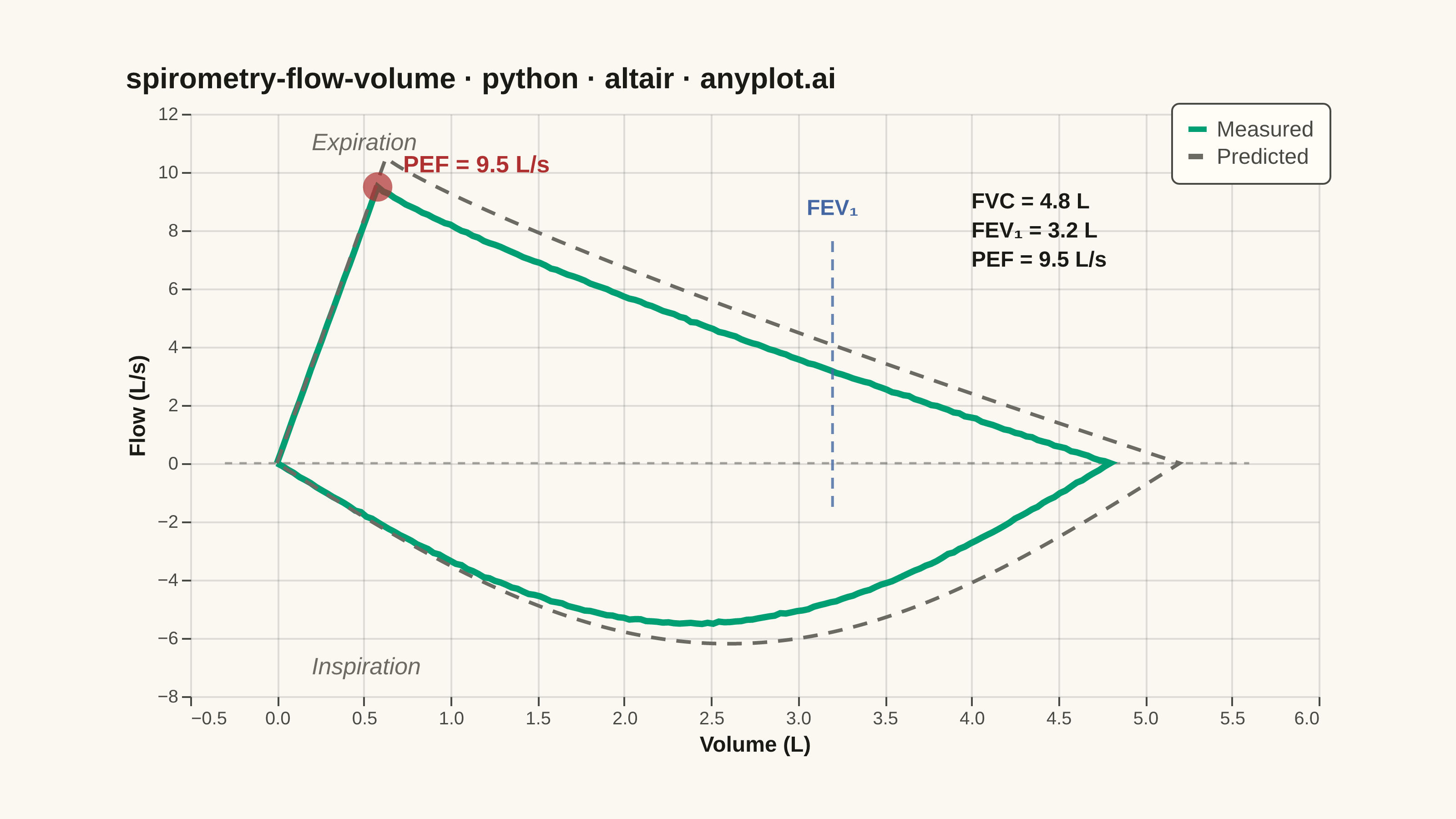
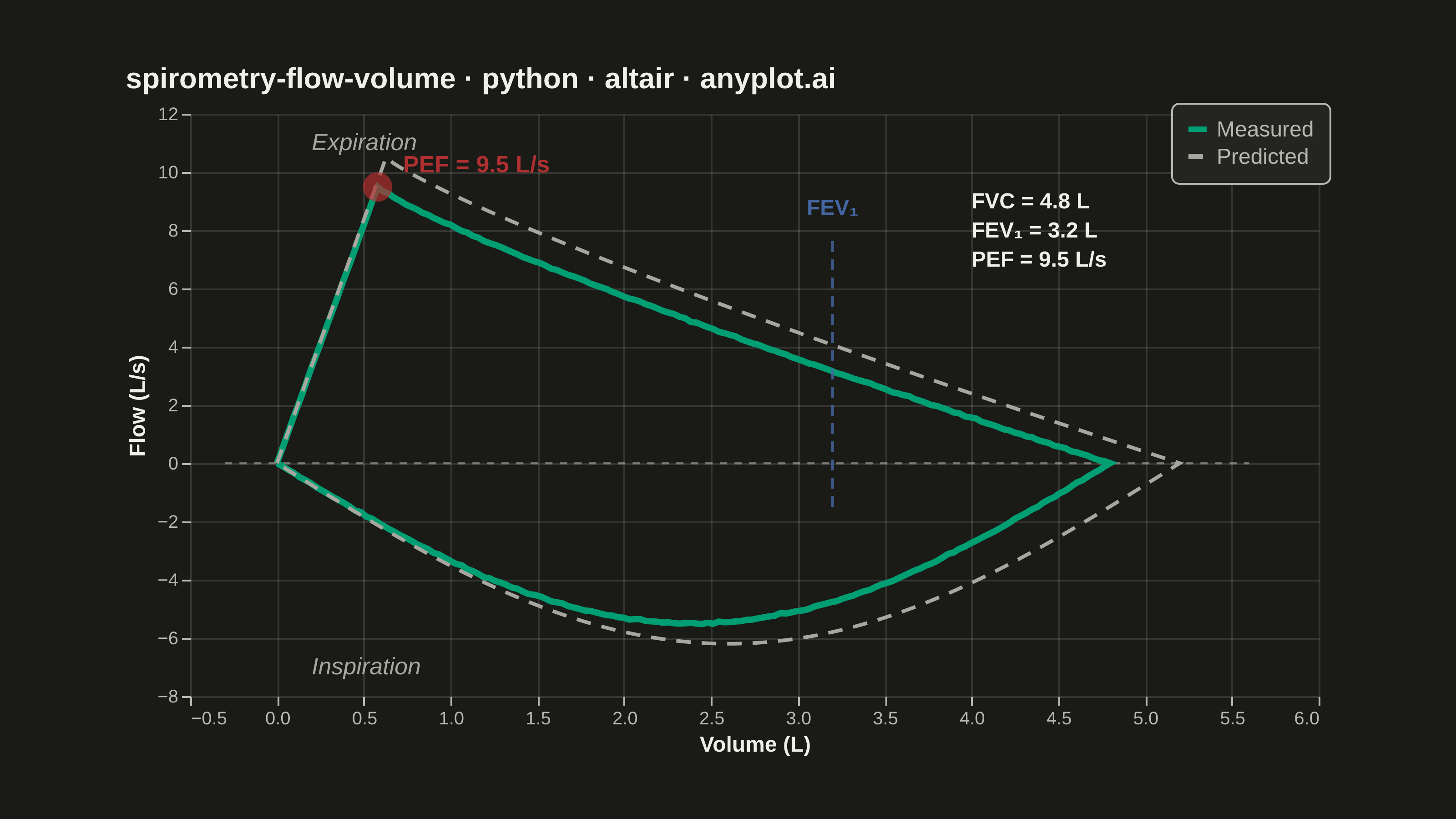
A pulmonary function test visualization that plots airflow rate (L/s) against lung volume (L) during forced expiration and inspiration, forming a characteristic loop shape. The expiratory limb rises sharply to Peak Expiratory Flow (PEF) then declines, while the inspiratory limb forms a more symmetric curve below the x-axis. This plot is essential for diagnosing obstructive and restrictive lung diseases by comparing measured loops against predicted normal values.
""" anyplot.ai
spirometry-flow-volume: Spirometry Flow-Volume Loop
Library: altair 6.2.1 | Python 3.13.13
Quality: 93/100 | Updated: 2026-06-17
"""

import os
import sys


# Remove script directory from sys.path to avoid importing local altair.py
_script_dir = os.path.dirname(os.path.abspath(__file__))
if _script_dir in sys.path:
    sys.path.remove(_script_dir)
# Also strip the '' / '.' empty-string entry added when running from this dir
sys.path[:] = [p for p in sys.path if os.path.abspath(p or ".") != _script_dir]

import altair as alt
import numpy as np
import pandas as pd
from PIL import Image


# Theme tokens (see prompts/default-style-guide.md "Theme-adaptive Chrome")
THEME = os.getenv("ANYPLOT_THEME", "light")
PAGE_BG = "#FAF8F1" if THEME == "light" else "#1A1A17"
ELEVATED_BG = "#FFFDF6" if THEME == "light" else "#242420"
INK = "#1A1A17" if THEME == "light" else "#F0EFE8"
INK_SOFT = "#4A4A44" if THEME == "light" else "#B8B7B0"
INK_MUTED = "#6B6A63" if THEME == "light" else "#A8A79F"

# Imprint palette — data colors stay identical across themes
BRAND = "#009E73"  # measured loop — ALWAYS first series
PREDICTED = INK_MUTED  # predicted normal overlay — theme-adaptive muted
PEF_RED = "#AE3030"  # Imprint matte red — focal Peak Expiratory Flow marker
FEV1_BLUE = "#4467A3"  # Imprint blue — FEV1 reference

# Data
np.random.seed(42)

fvc_measured = 4.8
fev1_measured = 3.2
pef_measured = 9.5
fvc_predicted = 5.2
pef_predicted = 10.5
n_points = 150

# Measured expiratory limb: sharp rise to PEF then linear decline
vol_exp = np.linspace(0, fvc_measured, n_points)
pef_idx = int(n_points * 0.12)
flow_rise = np.linspace(0, pef_measured, pef_idx + 1)
vol_remaining = vol_exp[pef_idx:] - vol_exp[pef_idx]
vol_range = fvc_measured - vol_exp[pef_idx]
flow_decline = pef_measured * (1 - (vol_remaining / vol_range) ** 0.85)
flow_exp = np.concatenate([flow_rise, flow_decline[1:]])
flow_exp += np.random.normal(0, 0.015, len(flow_exp))  # subtle physiological noise
flow_exp = np.clip(flow_exp, 0, None)
flow_exp[0] = 0
flow_exp[-1] = 0

# Measured inspiratory limb: symmetric U-shape below the zero-flow line
vol_insp = np.linspace(fvc_measured, 0, n_points)
t_insp = np.linspace(0, np.pi, n_points)
flow_insp = -5.5 * np.sin(t_insp)
flow_insp += np.random.normal(0, 0.015, len(flow_insp))
flow_insp[0] = 0
flow_insp[-1] = 0

# Predicted expiratory limb
vol_pred_exp = np.linspace(0, fvc_predicted, n_points)
pred_pef_idx = int(n_points * 0.12)
pred_flow_rise = np.linspace(0, pef_predicted, pred_pef_idx + 1)
pred_vol_remaining = vol_pred_exp[pred_pef_idx:] - vol_pred_exp[pred_pef_idx]
pred_vol_range = fvc_predicted - vol_pred_exp[pred_pef_idx]
pred_flow_decline = pef_predicted * (1 - (pred_vol_remaining / pred_vol_range) ** 0.85)
flow_pred_exp = np.concatenate([pred_flow_rise, pred_flow_decline[1:]])
flow_pred_exp = np.clip(flow_pred_exp, 0, None)
flow_pred_exp[0] = 0
flow_pred_exp[-1] = 0

# Predicted inspiratory limb
vol_pred_insp = np.linspace(fvc_predicted, 0, n_points)
t_pred_insp = np.linspace(0, np.pi, n_points)
flow_pred_insp = -6.2 * np.sin(t_pred_insp)
flow_pred_insp[0] = 0
flow_pred_insp[-1] = 0

# Combine into dataframes
df_measured = pd.concat(
    [pd.DataFrame({"volume": vol_exp, "flow": flow_exp}), pd.DataFrame({"volume": vol_insp, "flow": flow_insp})],
    ignore_index=True,
)
df_measured["curve"] = "Measured"
df_measured["order"] = range(len(df_measured))

df_predicted = pd.concat(
    [
        pd.DataFrame({"volume": vol_pred_exp, "flow": flow_pred_exp}),
        pd.DataFrame({"volume": vol_pred_insp, "flow": flow_pred_insp}),
    ],
    ignore_index=True,
)
df_predicted["curve"] = "Predicted"
df_predicted["order"] = range(len(df_predicted))

df_all = pd.concat([df_measured, df_predicted], ignore_index=True)

# PEF annotation point
pef_vol = vol_exp[np.argmax(flow_exp)]
pef_flow = float(flow_exp.max())
df_pef = pd.DataFrame({"volume": [pef_vol], "flow": [pef_flow], "label": [f"PEF = {pef_flow:.1f} L/s"]})

# Clinical values annotation
df_clinical = pd.DataFrame(
    {
        "volume": [4.0],
        "flow": [9.0],
        "label": [f"FVC = {fvc_measured:.1f} L\nFEV₁ = {fev1_measured:.1f} L\nPEF = {pef_flow:.1f} L/s"],
    }
)

# FEV1 marker: vertical reference at the 1-second volume
df_fev1_line = pd.DataFrame({"volume": [fev1_measured, fev1_measured], "flow": [-1.5, 7.8]})
df_fev1_label = pd.DataFrame({"volume": [fev1_measured], "flow": [8.4], "label": ["FEV₁"]})

# Color and dash scales for the legend
color_scale = alt.Scale(domain=["Measured", "Predicted"], range=[BRAND, PREDICTED])
dash_scale = alt.Scale(domain=["Measured", "Predicted"], range=[[1, 0], [8, 6]])

# Nearest selection for interactive hover tooltip (Altair-distinctive)
nearest = alt.selection_point(nearest=True, on="pointerover", fields=["order"], empty=False)

x_axis = alt.X("volume:Q", title="Volume (L)", scale=alt.Scale(domain=[-0.3, 5.6]))
y_axis = alt.Y("flow:Q", title="Flow (L/s)", scale=alt.Scale(domain=[-8, 12]))

# Zero-flow reference line
df_zero = pd.DataFrame({"volume": [-0.3, 5.6], "flow": [0, 0]})
zero_line = (
    alt.Chart(df_zero)
    .mark_line(strokeWidth=1.2, strokeDash=[4, 4], color=INK_MUTED, opacity=0.6)
    .encode(x=x_axis, y=y_axis)
)

# Main loops with legend
curves = (
    alt.Chart(df_all)
    .mark_line()
    .encode(
        x=x_axis,
        y=y_axis,
        order="order:Q",
        color=alt.Color(
            "curve:N",
            title=None,
            scale=color_scale,
            legend=alt.Legend(labelFontSize=12, symbolStrokeWidth=3, orient="top-right", offset=-6),
        ),
        strokeDash=alt.StrokeDash("curve:N", title=None, scale=dash_scale, legend=None),
        strokeWidth=alt.condition(alt.datum.curve == "Measured", alt.value(3.5), alt.value(2)),
    )
)

# Interactive hover layer (Altair-distinctive: reveals flow/volume on the measured loop)
tooltip_points = (
    alt.Chart(df_measured)
    .mark_point(opacity=0, size=80)
    .encode(
        x="volume:Q",
        y="flow:Q",
        tooltip=[
            alt.Tooltip("volume:Q", title="Volume (L)", format=".2f"),
            alt.Tooltip("flow:Q", title="Flow (L/s)", format=".2f"),
        ],
    )
    .add_params(nearest)
)

hover_rule = (
    alt.Chart(df_measured)
    .mark_rule(color=INK_SOFT, strokeWidth=1, strokeDash=[3, 3])
    .encode(x="volume:Q")
    .transform_filter(nearest)
)

hover_point = (
    alt.Chart(df_measured)
    .mark_point(size=120, filled=True, color=BRAND)
    .encode(x="volume:Q", y="flow:Q")
    .transform_filter(nearest)
)

# PEF focal marker and label
pef_point = alt.Chart(df_pef).mark_point(size=260, filled=True, color=PEF_RED).encode(x="volume:Q", y="flow:Q")
pef_label = (
    alt.Chart(df_pef)
    .mark_text(align="left", dx=14, dy=-12, fontSize=13, fontWeight="bold", color=PEF_RED)
    .encode(x="volume:Q", y="flow:Q", text="label:N")
)

# FEV1 vertical reference line with label
fev1_line = (
    alt.Chart(df_fev1_line)
    .mark_line(strokeWidth=1.5, strokeDash=[6, 4], color=FEV1_BLUE, opacity=0.8)
    .encode(x="volume:Q", y="flow:Q")
)
fev1_label = (
    alt.Chart(df_fev1_label)
    .mark_text(fontSize=12, fontWeight="bold", color=FEV1_BLUE, dy=-6)
    .encode(x="volume:Q", y="flow:Q", text="label:N")
)

# Clinical values text block
clinical_text = (
    alt.Chart(df_clinical)
    .mark_text(align="left", fontSize=12, lineBreak="\n", lineHeight=16, color=INK, fontWeight="bold")
    .encode(x="volume:Q", y="flow:Q", text="label:N")
)

# Expiratory / Inspiratory region labels (bumped up from the previous 14pt-equivalent)
df_region_exp = pd.DataFrame({"volume": [0.2], "flow": [11.0], "label": ["Expiration"]})
df_region_insp = pd.DataFrame({"volume": [0.2], "flow": [-7.0], "label": ["Inspiration"]})
region_exp_label = (
    alt.Chart(df_region_exp)
    .mark_text(fontSize=13, color=INK_MUTED, fontStyle="italic", align="left")
    .encode(x="volume:Q", y="flow:Q", text="label:N")
)
region_insp_label = (
    alt.Chart(df_region_insp)
    .mark_text(fontSize=13, color=INK_MUTED, fontStyle="italic", align="left")
    .encode(x="volume:Q", y="flow:Q", text="label:N")
)

# Title — scale fontsize off the 67-char baseline (this title is shorter, so stays at 16)
title_text = "spirometry-flow-volume · python · altair · anyplot.ai"
title_fontsize = round(16 * min(1.0, 67 / len(title_text)))

chart = (
    (
        zero_line
        + curves
        + tooltip_points
        + hover_rule
        + hover_point
        + fev1_line
        + fev1_label
        + pef_point
        + pef_label
        + clinical_text
        + region_exp_label
        + region_insp_label
    )
    .properties(
        width=620,
        height=320,
        background=PAGE_BG,
        title=alt.Title(title_text, fontSize=title_fontsize, anchor="start", color=INK),
    )
    .configure_view(fill=PAGE_BG, stroke=None)
    .configure_axis(
        labelFontSize=10,
        titleFontSize=12,
        domain=False,
        gridColor=INK,
        gridOpacity=0.12,
        tickColor=INK_SOFT,
        labelColor=INK_SOFT,
        titleColor=INK,
    )
    .configure_legend(
        labelFontSize=12, fillColor=ELEVATED_BG, strokeColor=INK_SOFT, labelColor=INK_SOFT, padding=8, cornerRadius=4
    )
)

# Save — altair view dims are not the saved PNG; pad up to the canonical 3200×1800
chart.save(f"plot-{THEME}.png", scale_factor=4.0)
chart.save(f"plot-{THEME}.html")

TW, TH = 3200, 1800
_img = Image.open(f"plot-{THEME}.png").convert("RGB")
_w, _h = _img.size
if _w > TW or _h > TH:
    raise SystemExit(
        f"altair vl-convert produced {_w}×{_h}, exceeds target {TW}×{TH}. "
        f"Shrink chart .properties(width=, height=) values and re-render."
    )
if _w < TW or _h < TH:
    _canvas = Image.new("RGB", (TW, TH), PAGE_BG)
    _canvas.paste(_img, ((TW - _w) // 2, (TH - _h) // 2))
    _canvas.save(f"plot-{THEME}.png")
Runnable source as JSON, for any HTTP client: https://api.anyplot.ai/specs/spirometry-flow-volume/altair/code. Any spec id and library id listed in llms-full.txt fit the same URL shape; every URL below is complete and callable.
{
  "spec_id": "spirometry-flow-volume",
  "language": "python",
  "library": "altair",
  "page": "https://anyplot.ai/spirometry-flow-volume/python/altair",
  "hub": "https://anyplot.ai/spirometry-flow-volume",
  "code_json": "https://api.anyplot.ai/specs/spirometry-flow-volume/altair/code",
  "spec_json": "https://api.anyplot.ai/specs/spirometry-flow-volume",
  "render_light_png": "https://storage.googleapis.com/anyplot-images/plots/spirometry-flow-volume/python/altair/plot-light.png",
  "render_dark_png": "https://storage.googleapis.com/anyplot-images/plots/spirometry-flow-volume/python/altair/plot-dark.png",
  "interactive_light_html": "https://storage.googleapis.com/anyplot-images/plots/spirometry-flow-volume/python/altair/plot-light.html",
  "interactive_dark_html": "https://storage.googleapis.com/anyplot-images/plots/spirometry-flow-volume/python/altair/plot-dark.html",
  "quality_score": 93.0,
  "license": "MIT",
  "guide": "https://anyplot.ai/llms.txt"
}
Part of Spirometry Flow-Volume Loop on anyplot.ai.