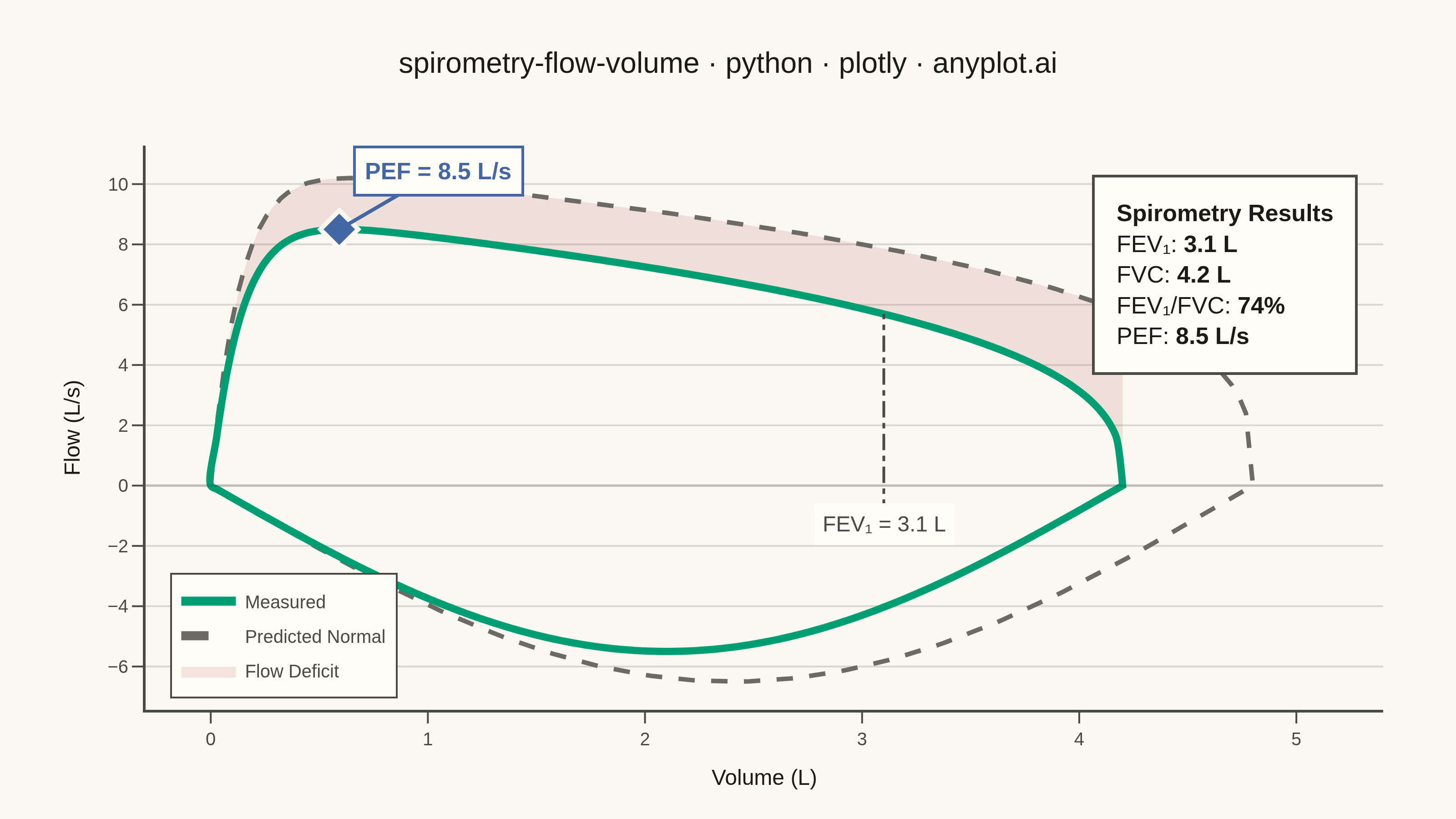
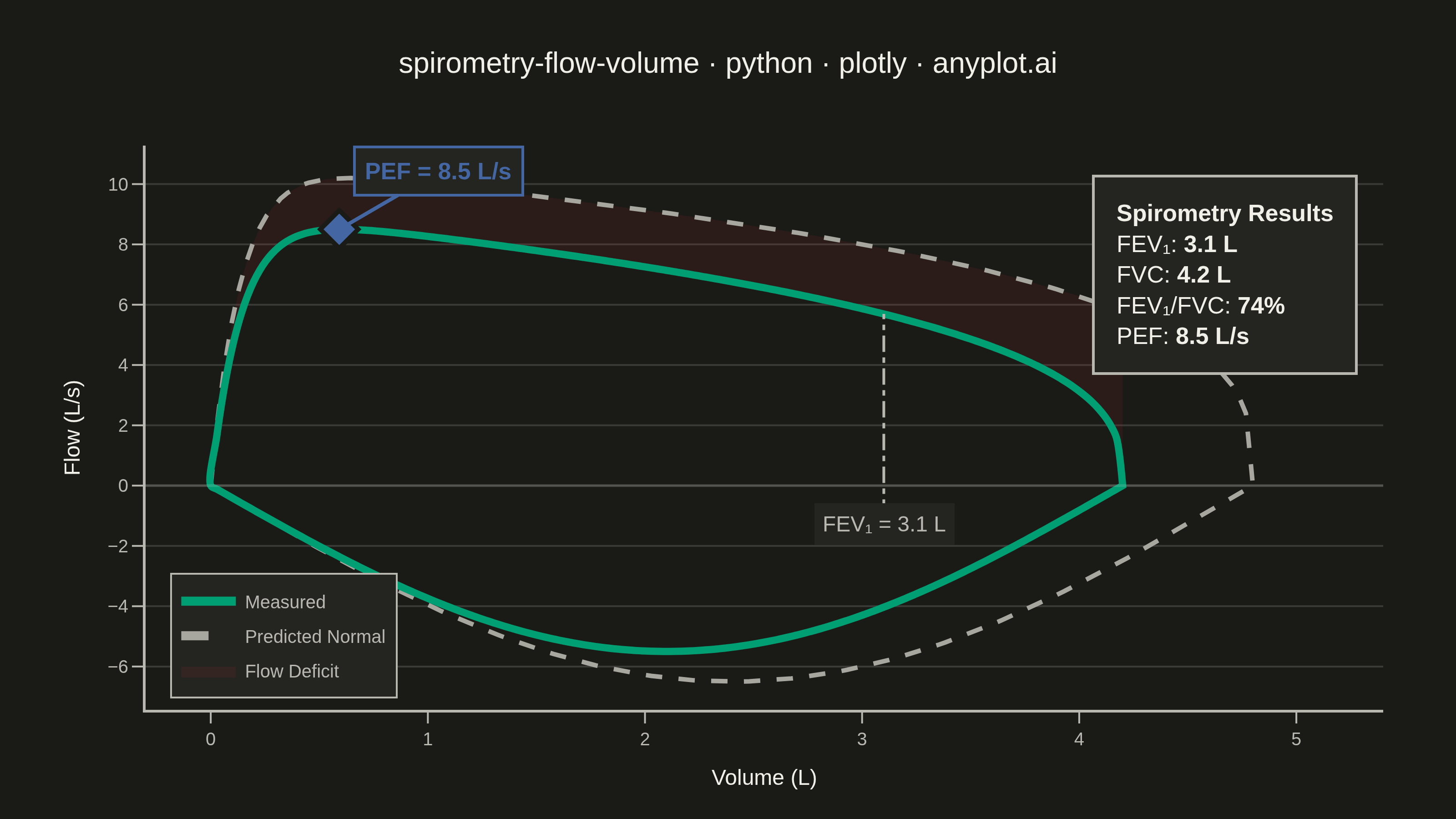
A pulmonary function test visualization that plots airflow rate (L/s) against lung volume (L) during forced expiration and inspiration, forming a characteristic loop shape. The expiratory limb rises sharply to Peak Expiratory Flow (PEF) then declines, while the inspiratory limb forms a more symmetric curve below the x-axis. This plot is essential for diagnosing obstructive and restrictive lung diseases by comparing measured loops against predicted normal values.
""" anyplot.ai
spirometry-flow-volume: Spirometry Flow-Volume Loop
Library: plotly 6.8.0 | Python 3.13.13
Quality: 94/100 | Updated: 2026-06-17
"""

import os

import numpy as np
import plotly.graph_objects as go


# Theme-adaptive chrome
THEME = os.getenv("ANYPLOT_THEME", "light")
PAGE_BG = "#FAF8F1" if THEME == "light" else "#1A1A17"
ELEVATED_BG = "#FFFDF6" if THEME == "light" else "#242420"
INK = "#1A1A17" if THEME == "light" else "#F0EFE8"
INK_SOFT = "#4A4A44" if THEME == "light" else "#B8B7B0"
INK_MUTED = "#6B6A63" if THEME == "light" else "#A8A79F"
GRID = "rgba(26,26,23,0.15)" if THEME == "light" else "rgba(240,239,232,0.15)"

# Imprint palette
BRAND = "#009E73"  # measured loop (always first series)
BLUE = "#4467A3"  # PEF landmark
MUTED = INK_MUTED  # predicted normal reference
# Flow deficit fill uses Imprint matte red #AE3030 (semantic: loss / obstruction) at low alpha

# Data - Spirometry flow-volume loop for a patient with mild obstruction
np.random.seed(42)

# Measured values
fvc = 4.2  # Forced Vital Capacity (L)
pef = 8.5  # Peak Expiratory Flow (L/s)
fev1 = 3.1  # FEV1 (L)

# Predicted normal values
fvc_pred = 4.8
pef_pred = 10.2

n_points = 150

# Expiratory limb: sharp rise to PEF then roughly linear decline.
# Normalised so the curve peak lands exactly on the stated PEF value.
volume_exp = np.linspace(0, fvc, n_points)
t_exp = volume_exp / fvc
flow_exp = (1 - t_exp) ** 0.35 * (1 - np.exp(-30 * t_exp))
flow_exp = np.maximum(flow_exp, 0)
flow_exp = flow_exp / flow_exp.max() * pef

# Inspiratory limb: symmetric U-shape below zero line
volume_insp = np.linspace(fvc, 0, n_points)
t_insp = np.linspace(0, 1, n_points)
pif = -5.5  # Peak Inspiratory Flow
flow_insp = pif * np.sin(np.pi * t_insp)

# Predicted normal expiratory limb (peak pinned to predicted PEF)
volume_pred_exp = np.linspace(0, fvc_pred, n_points)
t_pred_exp = volume_pred_exp / fvc_pred
flow_pred_exp = (1 - t_pred_exp) ** 0.3 * (1 - np.exp(-35 * t_pred_exp))
flow_pred_exp = np.maximum(flow_pred_exp, 0)
flow_pred_exp = flow_pred_exp / flow_pred_exp.max() * pef_pred

# Predicted normal inspiratory limb
volume_pred_insp = np.linspace(fvc_pred, 0, n_points)
t_pred_insp = np.linspace(0, 1, n_points)
pif_pred = -6.5
flow_pred_insp = pif_pred * np.sin(np.pi * t_pred_insp)

# Combine into closed loops
volume_measured = np.concatenate([volume_exp, volume_insp])
flow_measured = np.concatenate([flow_exp, flow_insp])

volume_predicted = np.concatenate([volume_pred_exp, volume_pred_insp])
flow_predicted = np.concatenate([flow_pred_exp, flow_pred_insp])

# PEF point now coincides exactly with the curve peak
pef_idx = np.argmax(flow_exp)
pef_volume = volume_exp[pef_idx]

# FEV1 volume marker
fev1_volume = fev1

# Plot
fig = go.Figure()

# Shaded deficit between predicted and measured expiratory curves (obstruction)
vol_common = np.linspace(0, min(fvc, fvc_pred), 120)
flow_pred_interp = np.interp(vol_common, volume_pred_exp, flow_pred_exp)
flow_meas_interp = np.interp(vol_common, volume_exp, flow_exp)

fig.add_trace(
    go.Scatter(
        x=np.concatenate([vol_common, vol_common[::-1]]),
        y=np.concatenate([flow_pred_interp, flow_meas_interp[::-1]]),
        fill="toself",
        fillcolor="rgba(174, 48, 48, 0.12)",
        line={"width": 0},
        name="Flow Deficit",
        showlegend=True,
        hoverinfo="skip",
        legendrank=3,
    )
)

# Predicted normal loop (dashed reference, behind measured)
fig.add_trace(
    go.Scatter(
        x=volume_predicted,
        y=flow_predicted,
        mode="lines",
        line={"color": MUTED, "width": 2.5, "dash": "dash"},
        name="Predicted Normal",
        hovertemplate="<b>Predicted</b><br>Volume: %{x:.2f} L<br>Flow: %{y:.2f} L/s<extra></extra>",
        legendrank=2,
    )
)

# Measured loop (solid brand green)
fig.add_trace(
    go.Scatter(
        x=volume_measured,
        y=flow_measured,
        mode="lines",
        line={"color": BRAND, "width": 4, "shape": "spline"},
        name="Measured",
        hovertemplate="<b>Measured</b><br>Volume: %{x:.2f} L<br>Flow: %{y:.2f} L/s<extra></extra>",
        legendrank=1,
    )
)

# PEF marker sitting exactly on the curve peak
fig.add_trace(
    go.Scatter(
        x=[pef_volume],
        y=[pef],
        mode="markers",
        marker={"size": 16, "color": BLUE, "symbol": "diamond", "line": {"width": 2.5, "color": PAGE_BG}},
        name="PEF",
        showlegend=False,
        hovertemplate="<b>Peak Expiratory Flow</b><br>%{y:.1f} L/s at %{x:.2f} L<extra></extra>",
    )
)

# PEF annotation with arrow
fig.add_annotation(
    x=pef_volume,
    y=pef,
    text=f"<b>PEF = {pef:.1f} L/s</b>",
    showarrow=True,
    arrowhead=0,
    arrowwidth=2,
    arrowcolor=BLUE,
    ax=55,
    ay=-32,
    font={"size": 13, "color": BLUE},
    bgcolor=ELEVATED_BG,
    bordercolor=BLUE,
    borderwidth=1.5,
    borderpad=5,
)

# FEV1 vertical reference line
fig.add_shape(
    type="line",
    x0=fev1_volume,
    x1=fev1_volume,
    y0=-1,
    y1=np.interp(fev1_volume, volume_exp, flow_exp),
    line={"color": INK_SOFT, "width": 1.5, "dash": "dashdot"},
)

fig.add_annotation(
    x=fev1_volume,
    y=-1.3,
    text=f"FEV₁ = {fev1:.1f} L",
    showarrow=False,
    font={"size": 12, "color": INK_SOFT},
    bgcolor=ELEVATED_BG,
    borderpad=4,
)

# Clinical values annotation box
clinical_text = (
    f"<b>Spirometry Results</b><br>"
    f"FEV₁: <b>{fev1:.1f} L</b><br>"
    f"FVC: <b>{fvc:.1f} L</b><br>"
    f"FEV₁/FVC: <b>{fev1 / fvc:.0%}</b><br>"
    f"PEF: <b>{pef:.1f} L/s</b>"
)
fig.add_annotation(
    x=0.98,
    y=0.95,
    xref="paper",
    yref="paper",
    text=clinical_text,
    showarrow=False,
    font={"size": 13, "color": INK},
    align="left",
    bordercolor=INK_SOFT,
    borderwidth=1.5,
    borderpad=12,
    bgcolor=ELEVATED_BG,
    xanchor="right",
    yanchor="top",
)

# Zero flow reference line
fig.add_hline(y=0, line={"color": GRID, "width": 1.5})

# Layout
fig.update_layout(
    autosize=False,
    title={
        "text": "spirometry-flow-volume · python · plotly · anyplot.ai",
        "font": {"size": 16, "color": INK},
        "x": 0.5,
        "xanchor": "center",
    },
    xaxis={
        "title": {"text": "Volume (L)", "font": {"size": 12, "color": INK}, "standoff": 12},
        "tickfont": {"size": 10, "color": INK_SOFT},
        "showgrid": False,
        "zeroline": False,
        "range": [-0.3, max(fvc, fvc_pred) + 0.6],
        "linecolor": INK_SOFT,
        "linewidth": 1.5,
        "ticks": "outside",
        "ticklen": 6,
        "tickcolor": INK_SOFT,
        "dtick": 1,
    },
    yaxis={
        "title": {"text": "Flow (L/s)", "font": {"size": 12, "color": INK}, "standoff": 12},
        "tickfont": {"size": 10, "color": INK_SOFT},
        "showgrid": True,
        "gridcolor": GRID,
        "gridwidth": 1,
        "zeroline": False,
        "linecolor": INK_SOFT,
        "linewidth": 1.5,
        "ticks": "outside",
        "ticklen": 6,
        "tickcolor": INK_SOFT,
        "dtick": 2,
    },
    legend={
        "font": {"size": 10, "color": INK_SOFT},
        "x": 0.02,
        "y": 0.02,
        "xanchor": "left",
        "yanchor": "bottom",
        "bgcolor": ELEVATED_BG,
        "bordercolor": INK_SOFT,
        "borderwidth": 1,
        "itemsizing": "constant",
        "tracegroupgap": 4,
    },
    margin={"l": 80, "r": 40, "t": 80, "b": 60},
    paper_bgcolor=PAGE_BG,
    plot_bgcolor=PAGE_BG,
    hoverlabel={"bgcolor": ELEVATED_BG, "bordercolor": BRAND, "font": {"size": 12, "color": INK}},
    hovermode="closest",
)

# Save
fig.write_image(f"plot-{THEME}.png", width=800, height=450, scale=4)
fig.write_html(f"plot-{THEME}.html", include_plotlyjs="cdn")
Runnable source as JSON, for any HTTP client: https://api.anyplot.ai/specs/spirometry-flow-volume/plotly/code. Any spec id and library id listed in llms-full.txt fit the same URL shape; every URL below is complete and callable.
{
  "spec_id": "spirometry-flow-volume",
  "language": "python",
  "library": "plotly",
  "page": "https://anyplot.ai/spirometry-flow-volume/python/plotly",
  "hub": "https://anyplot.ai/spirometry-flow-volume",
  "code_json": "https://api.anyplot.ai/specs/spirometry-flow-volume/plotly/code",
  "spec_json": "https://api.anyplot.ai/specs/spirometry-flow-volume",
  "render_light_png": "https://storage.googleapis.com/anyplot-images/plots/spirometry-flow-volume/python/plotly/plot-light.png",
  "render_dark_png": "https://storage.googleapis.com/anyplot-images/plots/spirometry-flow-volume/python/plotly/plot-dark.png",
  "interactive_light_html": "https://storage.googleapis.com/anyplot-images/plots/spirometry-flow-volume/python/plotly/plot-light.html",
  "interactive_dark_html": "https://storage.googleapis.com/anyplot-images/plots/spirometry-flow-volume/python/plotly/plot-dark.html",
  "quality_score": 94.0,
  "license": "MIT",
  "guide": "https://anyplot.ai/llms.txt"
}
Part of Spirometry Flow-Volume Loop on anyplot.ai.