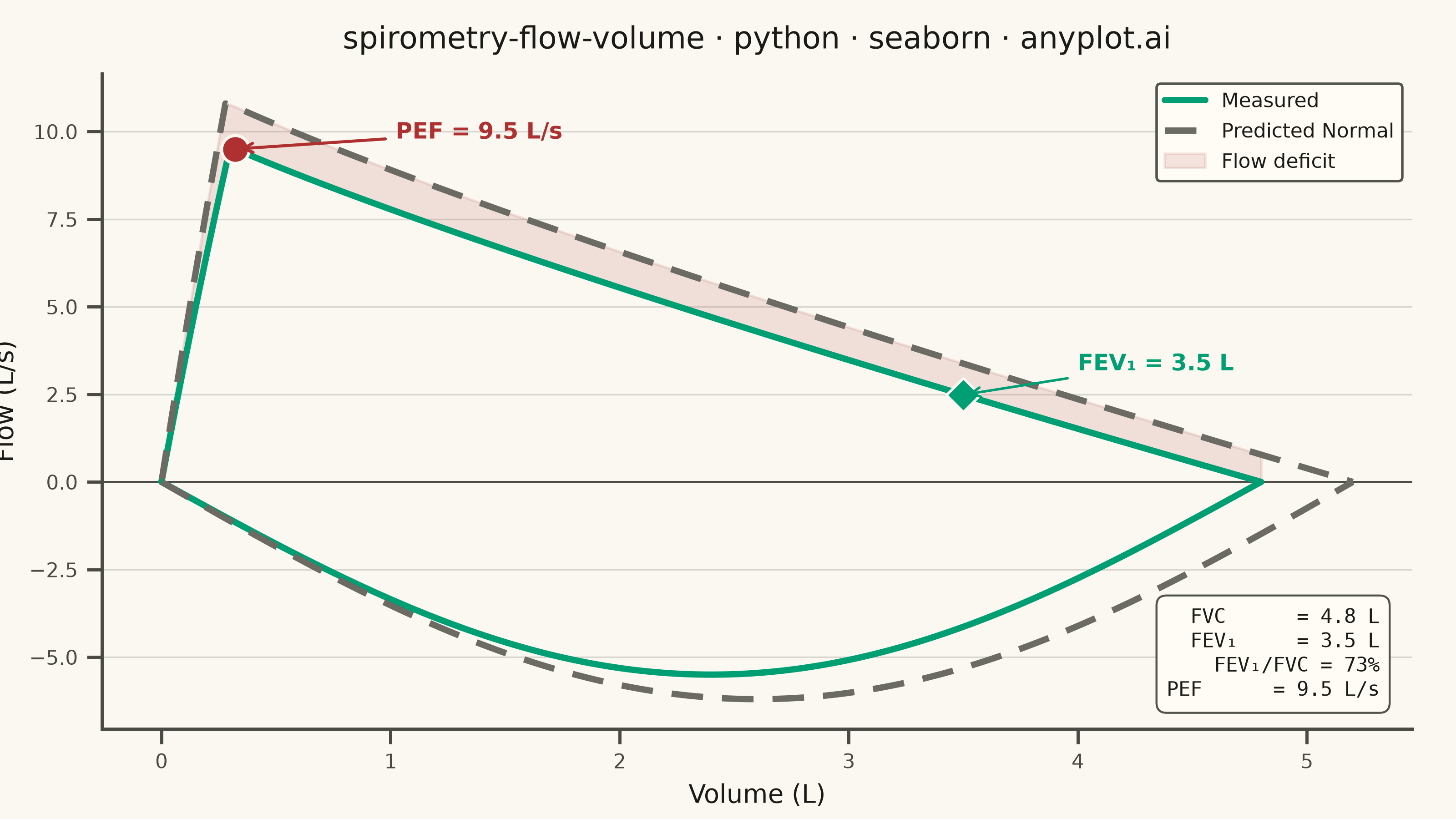
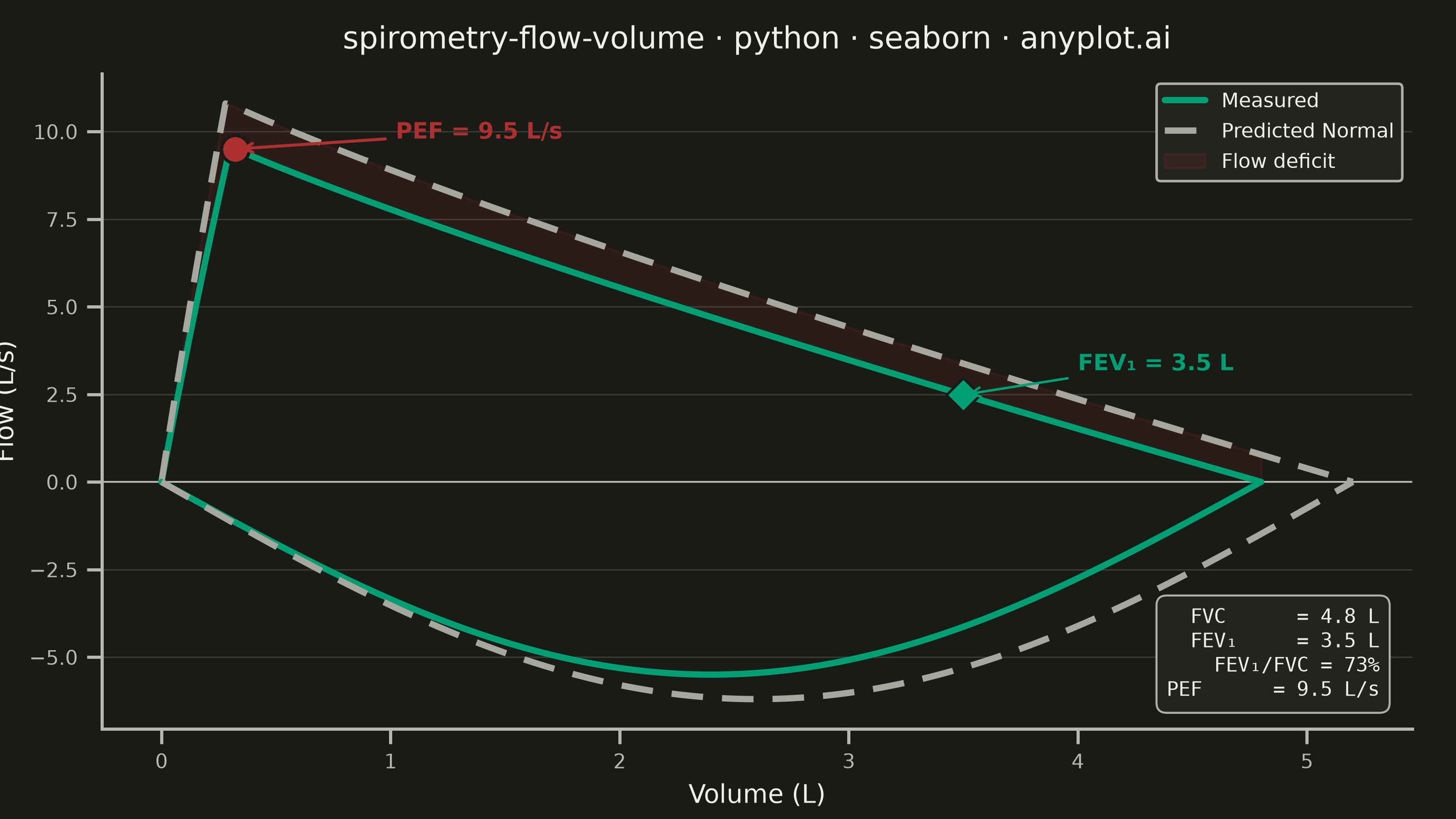
A pulmonary function test visualization that plots airflow rate (L/s) against lung volume (L) during forced expiration and inspiration, forming a characteristic loop shape. The expiratory limb rises sharply to Peak Expiratory Flow (PEF) then declines, while the inspiratory limb forms a more symmetric curve below the x-axis. This plot is essential for diagnosing obstructive and restrictive lung diseases by comparing measured loops against predicted normal values.
""" anyplot.ai
spirometry-flow-volume: Spirometry Flow-Volume Loop
Library: seaborn 0.13.2 | Python 3.13.13
Quality: 92/100 | Updated: 2026-06-17
"""

import os

import matplotlib.pyplot as plt
import numpy as np
import pandas as pd
import seaborn as sns


# Theme-adaptive chrome (Imprint palette)
THEME = os.getenv("ANYPLOT_THEME", "light")
PAGE_BG = "#FAF8F1" if THEME == "light" else "#1A1A17"
ELEVATED_BG = "#FFFDF6" if THEME == "light" else "#242420"
INK = "#1A1A17" if THEME == "light" else "#F0EFE8"
INK_SOFT = "#4A4A44" if THEME == "light" else "#B8B7B0"
INK_MUTED = "#6B6A63" if THEME == "light" else "#A8A79F"

# Imprint categorical palette + semantic anchors
BRAND = "#009E73"  # brand green — measured loop (first series)
LOSS = "#AE3030"  # matte red — semantic anchor for flow deficit / shortfall
PREDICTED = INK_MUTED  # muted neutral — reference / predicted-normal overlay

# Data
np.random.seed(42)

fvc_measured = 4.8
pef_measured = 9.5
fev1_measured = 3.5

n_points = 150

# Expiratory limb (positive flow): sharp rise to PEF then linear decline
vol_exp = np.linspace(0, fvc_measured, n_points)
rise_phase = np.minimum(vol_exp / 0.3, 1.0)
decay_phase = 1.0 - (vol_exp / fvc_measured) ** 0.85
flow_exp_raw = rise_phase * decay_phase
flow_exp = pef_measured * flow_exp_raw / flow_exp_raw.max()
flow_exp = np.maximum(flow_exp, 0)

# Inspiratory limb (negative flow): symmetric U-shaped curve
vol_insp = np.linspace(0, fvc_measured, n_points)
flow_insp = -5.5 * np.sin(np.linspace(np.pi, 0, n_points))

# Predicted normal values
fvc_predicted = 5.2
pef_predicted = 10.8
vol_pred_exp = np.linspace(0, fvc_predicted, n_points)
rise_pred = np.minimum(vol_pred_exp / 0.28, 1.0)
decay_pred = 1.0 - (vol_pred_exp / fvc_predicted) ** 0.85
flow_pred_exp_raw = rise_pred * decay_pred
flow_pred_exp = pef_predicted * flow_pred_exp_raw / flow_pred_exp_raw.max()
flow_pred_exp = np.maximum(flow_pred_exp, 0)

vol_pred_insp = np.linspace(0, fvc_predicted, n_points)
flow_pred_insp = -6.2 * np.sin(np.linspace(np.pi, 0, n_points))

# Build DataFrame using a style column for idiomatic seaborn hue+style plotting
df = pd.DataFrame(
    {
        "Volume (L)": np.concatenate([vol_exp, vol_insp, vol_pred_exp, vol_pred_insp]),
        "Flow (L/s)": np.concatenate([flow_exp, flow_insp, flow_pred_exp, flow_pred_insp]),
        "Curve": (
            ["Measured"] * n_points
            + ["Measured"] * n_points
            + ["Predicted Normal"] * n_points
            + ["Predicted Normal"] * n_points
        ),
        "Limb": (
            ["Expiratory"] * n_points
            + ["Inspiratory"] * n_points
            + ["Expiratory"] * n_points
            + ["Inspiratory"] * n_points
        ),
    }
)

# seaborn theming — theme-adaptive chrome
sns.set_theme(
    style="ticks",
    rc={
        "figure.facecolor": PAGE_BG,
        "axes.facecolor": PAGE_BG,
        "axes.edgecolor": INK_SOFT,
        "axes.labelcolor": INK,
        "text.color": INK,
        "xtick.color": INK_SOFT,
        "ytick.color": INK_SOFT,
        "grid.color": INK,
        "grid.alpha": 0.15,
        "legend.facecolor": ELEVATED_BG,
        "legend.edgecolor": INK_SOFT,
    },
)

# Canvas — hard rule: 8 × 4.5 in @ 400 dpi = 3200 × 1800 px
fig, ax = plt.subplots(figsize=(8, 4.5), dpi=400)

# Plot using sns.lineplot with hue AND style for idiomatic seaborn dash control.
# style drives the dash pattern natively without post-hoc artist iteration.
for limb_name in ["Expiratory", "Inspiratory"]:
    limb_df = df[df["Limb"] == limb_name]
    sns.lineplot(
        data=limb_df,
        x="Volume (L)",
        y="Flow (L/s)",
        hue="Curve",
        style="Curve",
        palette={"Measured": BRAND, "Predicted Normal": PREDICTED},
        dashes={"Measured": "", "Predicted Normal": (5, 3)},
        linewidth=2.5,
        ax=ax,
        legend=(limb_name == "Expiratory"),
    )

# Shade flow deficit between measured and predicted expiratory limbs
vol_shade = np.linspace(0, min(fvc_measured, fvc_predicted), 200)
flow_meas_interp = np.interp(vol_shade, vol_exp, flow_exp)
flow_pred_interp = np.interp(vol_shade, vol_pred_exp, flow_pred_exp)
ax.fill_between(vol_shade, flow_meas_interp, flow_pred_interp, alpha=0.12, color=LOSS, label="Flow deficit", zorder=1)

# Mark PEF (peak expiratory flow) — the clinical highlight on the measured curve
pef_idx = np.argmax(flow_exp)
pef_actual = flow_exp[pef_idx]
pef_df = pd.DataFrame({"Volume (L)": [vol_exp[pef_idx]], "Flow (L/s)": [pef_actual]})
sns.scatterplot(
    data=pef_df,
    x="Volume (L)",
    y="Flow (L/s)",
    color=LOSS,
    s=120,
    zorder=5,
    edgecolor=PAGE_BG,
    linewidth=1.2,
    legend=False,
    ax=ax,
)
ax.annotate(
    f"PEF = {pef_actual:.1f} L/s",
    xy=(vol_exp[pef_idx], pef_actual),
    xytext=(vol_exp[pef_idx] + 0.7, pef_actual + 0.3),
    fontsize=9,
    fontweight="bold",
    color=LOSS,
    arrowprops={"arrowstyle": "->", "color": LOSS, "lw": 1.2},
    zorder=5,
)

# Mark FEV1 point on the measured expiratory curve
fev1_flow = np.interp(fev1_measured, vol_exp, flow_exp)
fev1_df = pd.DataFrame({"Volume (L)": [fev1_measured], "Flow (L/s)": [fev1_flow]})
sns.scatterplot(
    data=fev1_df,
    x="Volume (L)",
    y="Flow (L/s)",
    color=BRAND,
    marker="D",
    s=90,
    zorder=5,
    edgecolor=PAGE_BG,
    linewidth=1.0,
    legend=False,
    ax=ax,
)
ax.annotate(
    f"FEV₁ = {fev1_measured:.1f} L",
    xy=(fev1_measured, fev1_flow),
    xytext=(fev1_measured + 0.5, fev1_flow + 0.7),
    fontsize=9,
    fontweight="semibold",
    color=BRAND,
    arrowprops={"arrowstyle": "->", "color": BRAND, "lw": 1.0},
    zorder=5,
)

# Clinical values callout box
fev1_fvc_ratio = fev1_measured / fvc_measured * 100
textstr = (
    f"FVC      = {fvc_measured:.1f} L\n"
    f"FEV₁     = {fev1_measured:.1f} L\n"
    f"FEV₁/FVC = {fev1_fvc_ratio:.0f}%\n"
    f"PEF      = {pef_actual:.1f} L/s"
)
props = {"boxstyle": "round,pad=0.5", "facecolor": ELEVATED_BG, "edgecolor": INK_SOFT, "alpha": 0.95, "linewidth": 0.8}
ax.text(
    0.975,
    0.04,
    textstr,
    transform=ax.transAxes,
    fontsize=8,
    color=INK,
    verticalalignment="bottom",
    horizontalalignment="right",
    bbox=props,
    family="monospace",
    zorder=6,
)

# Zero-flow reference line separating expiratory and inspiratory limbs
ax.axhline(y=0, color=INK_SOFT, linewidth=0.7, linestyle="-", zorder=1)

# Labels and title
ax.set_xlabel("Volume (L)", fontsize=10)
ax.set_ylabel("Flow (L/s)", fontsize=10)
ax.set_title(
    "spirometry-flow-volume · python · seaborn · anyplot.ai", fontsize=12, fontweight="medium", color=INK, pad=10
)
ax.tick_params(axis="both", labelsize=8)
ax.yaxis.grid(True, alpha=0.15, linewidth=0.6)
ax.xaxis.grid(False)
sns.despine(ax=ax)

# Single legend pass (measured, predicted, flow deficit) — no redundant override
handles, labels = ax.get_legend_handles_labels()
legend = ax.legend(handles=handles, labels=labels, fontsize=8, loc="upper right", framealpha=0.95)
legend.get_frame().set_facecolor(ELEVATED_BG)
legend.get_frame().set_edgecolor(INK_SOFT)
for text in legend.get_texts():
    text.set_color(INK)

fig.subplots_adjust(left=0.07, right=0.97, top=0.91, bottom=0.11)
plt.savefig(f"plot-{THEME}.png", dpi=400, facecolor=PAGE_BG)
Runnable source as JSON, for any HTTP client: https://api.anyplot.ai/specs/spirometry-flow-volume/seaborn/code. Any spec id and library id listed in llms-full.txt fit the same URL shape; every URL below is complete and callable.
{
  "spec_id": "spirometry-flow-volume",
  "language": "python",
  "library": "seaborn",
  "page": "https://anyplot.ai/spirometry-flow-volume/python/seaborn",
  "hub": "https://anyplot.ai/spirometry-flow-volume",
  "code_json": "https://api.anyplot.ai/specs/spirometry-flow-volume/seaborn/code",
  "spec_json": "https://api.anyplot.ai/specs/spirometry-flow-volume",
  "render_light_png": "https://storage.googleapis.com/anyplot-images/plots/spirometry-flow-volume/python/seaborn/plot-light.png",
  "render_dark_png": "https://storage.googleapis.com/anyplot-images/plots/spirometry-flow-volume/python/seaborn/plot-dark.png",
  "quality_score": 92.0,
  "license": "MIT",
  "guide": "https://anyplot.ai/llms.txt"
}
Part of Spirometry Flow-Volume Loop on anyplot.ai.