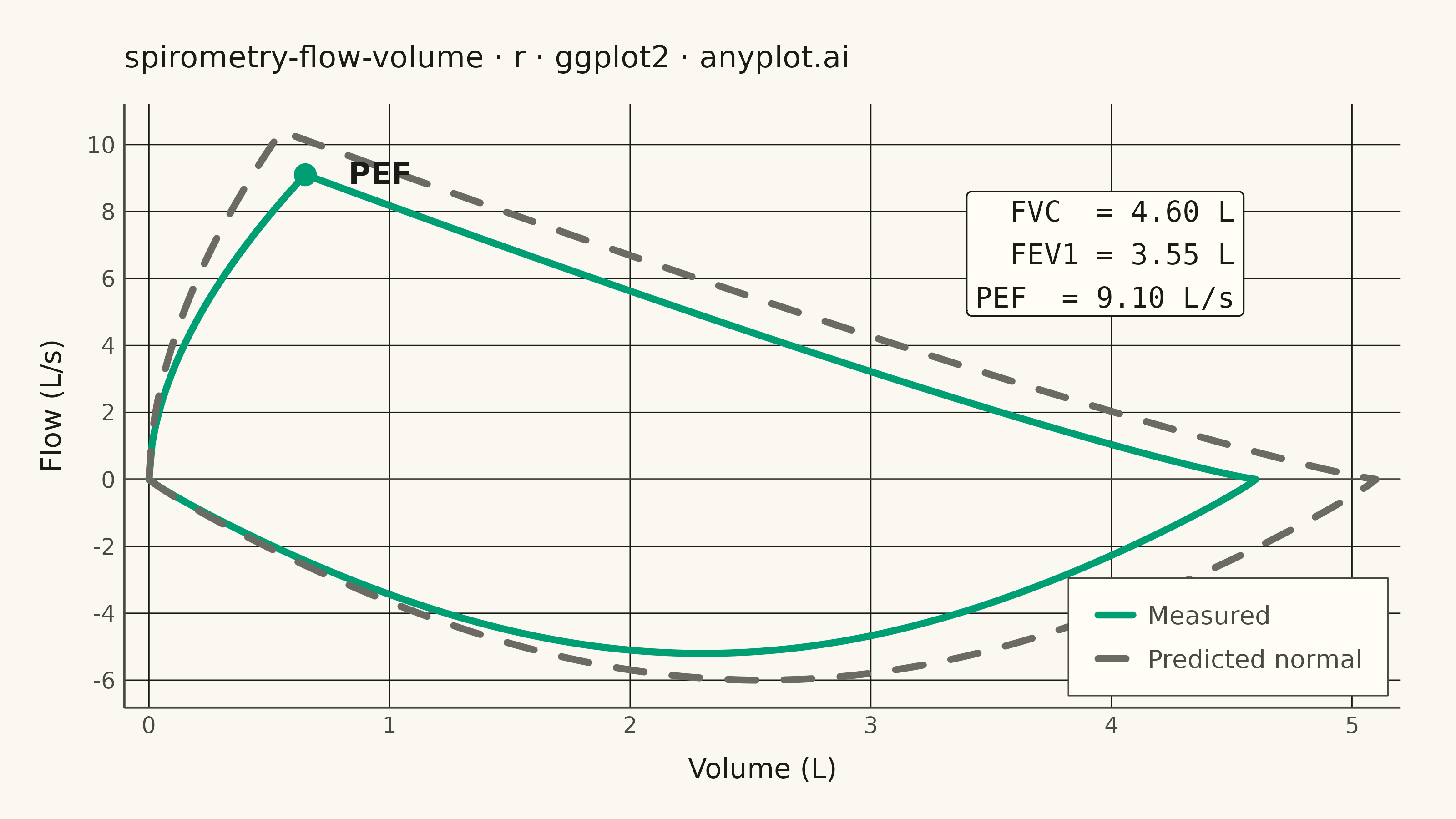
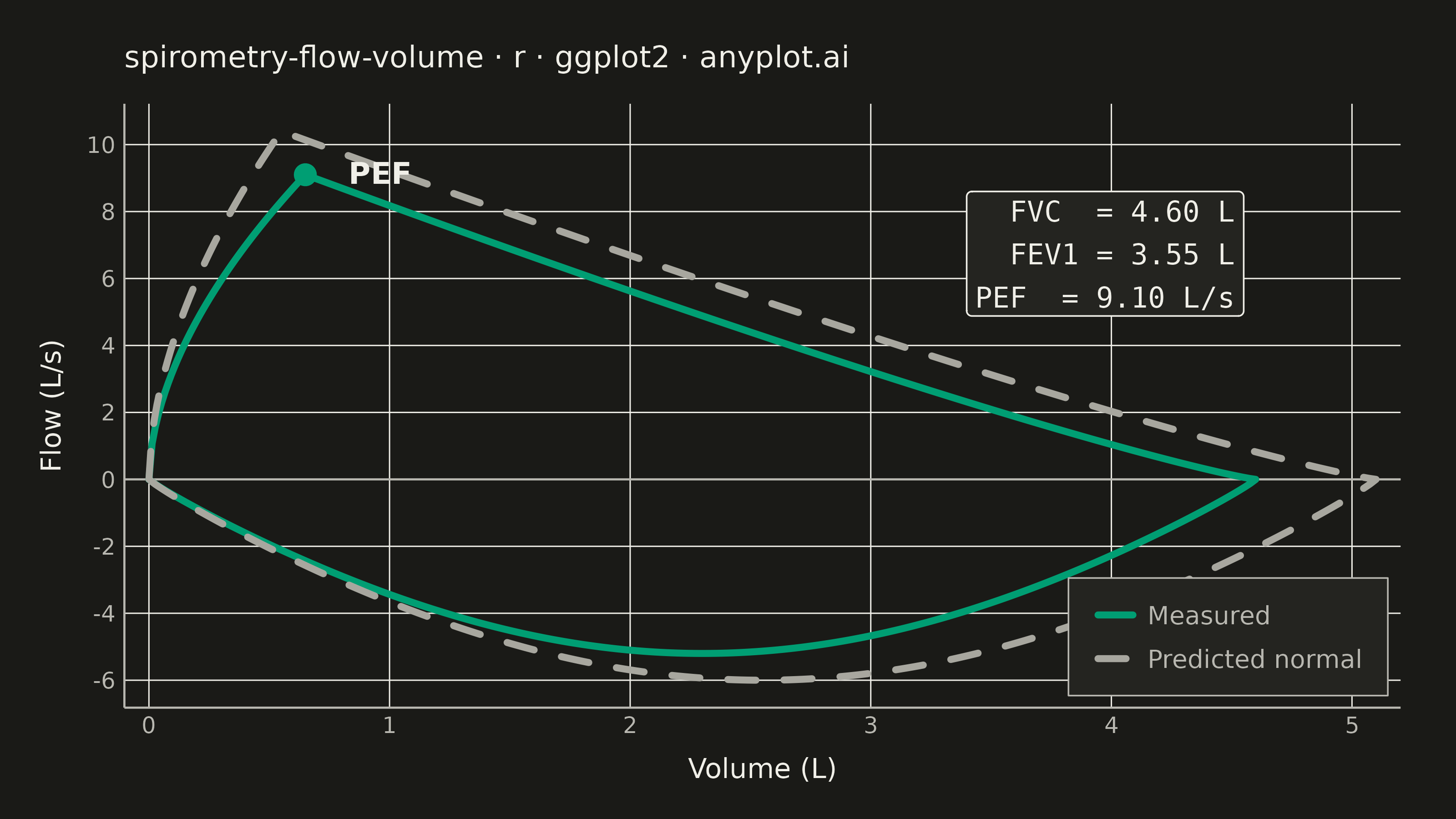
A pulmonary function test visualization that plots airflow rate (L/s) against lung volume (L) during forced expiration and inspiration, forming a characteristic loop shape. The expiratory limb rises sharply to Peak Expiratory Flow (PEF) then declines, while the inspiratory limb forms a more symmetric curve below the x-axis. This plot is essential for diagnosing obstructive and restrictive lung diseases by comparing measured loops against predicted normal values.
#' anyplot.ai
#' spirometry-flow-volume: Spirometry Flow-Volume Loop
#' Library: ggplot2 3.5.1 | R 4.4.1
#' Quality: 91/100 | Created: 2026-06-17

library(ggplot2)
library(dplyr)
library(ragg)

set.seed(42)

# --- Theme tokens -----------------------------------------------------------
THEME       <- Sys.getenv("ANYPLOT_THEME", "light")
PAGE_BG     <- if (THEME == "light") "#FAF8F1" else "#1A1A17"
ELEVATED_BG <- if (THEME == "light") "#FFFDF6" else "#242420"
INK         <- if (THEME == "light") "#1A1A17" else "#F0EFE8"
INK_SOFT    <- if (THEME == "light") "#4A4A44" else "#B8B7B0"
INK_MUTED   <- if (THEME == "light") "#6B6A63" else "#A8A79F"
GRID        <- if (THEME == "light") "#1A1A17" else "#F0EFE8"

BRAND <- "#009E73"  # Imprint palette position 1 — measured loop (first series)
MUTED <- INK_MUTED  # Imprint semantic anchor "muted" — predicted normal reference

# --- Data -------------------------------------------------------------------
# Forced spirometry maneuver: airflow (L/s) vs exhaled lung volume (L).
# Expiratory limb rises sharply to Peak Expiratory Flow (PEF) then declines
# roughly linearly; inspiratory limb is a symmetric U below the zero-flow line.
flow_volume_loop <- function(fvc, pef, pif, v_peak) {
    # Expiratory limb: 0 -> FVC, sharp rise to PEF then near-linear decline.
    v_rise <- seq(0, v_peak, length.out = 50)
    f_rise <- pef * (v_rise / v_peak)^0.55
    v_fall <- seq(v_peak, fvc, length.out = 150)[-1]
    f_fall <- pef * (1 - (v_fall - v_peak) / (fvc - v_peak))^1.15

    # Inspiratory limb: FVC -> 0, symmetric U-shaped curve (negative flow).
    v_insp <- seq(fvc, 0, length.out = 200)
    f_insp <- -pif * sin(pi * v_insp / fvc)^0.9

    data.frame(
        volume = c(v_rise, v_fall, v_insp),
        flow   = c(f_rise, f_fall, f_insp)
    )
}

# Predicted normal loop (reference) and the patient's measured loop.
predicted <- flow_volume_loop(fvc = 5.1, pef = 10.4, pif = 6.0, v_peak = 0.55) %>%
    mutate(series = "Predicted normal")
measured <- flow_volume_loop(fvc = 4.6, pef = 9.1, pif = 5.2, v_peak = 0.65) %>%
    mutate(series = "Measured")

loop_df <- bind_rows(measured, predicted) %>%
    mutate(series = factor(series, levels = c("Measured", "Predicted normal")))

# Peak Expiratory Flow marker (highest flow on the measured loop).
pef_point <- measured %>% slice_max(flow, n = 1)

# Clinical summary values for the measured maneuver.
clinical <- paste(
    "FVC  = 4.60 L",
    "FEV1 = 3.55 L",
    "PEF  = 9.10 L/s",
    sep = "\n"
)

# --- Plot -------------------------------------------------------------------
p <- ggplot(loop_df, aes(volume, flow, color = series, linetype = series)) +
    geom_hline(yintercept = 0, color = INK_SOFT, linewidth = 0.4) +
    geom_path(linewidth = 1.3, lineend = "round") +
    geom_point(
        data = pef_point, aes(volume, flow),
        inherit.aes = FALSE, color = BRAND, size = 3.6
    ) +
    annotate(
        "text", x = pef_point$volume + 0.18, y = pef_point$flow + 0.05,
        label = "PEF", hjust = 0, vjust = 0.5,
        color = INK, size = 4.2, fontface = "bold"
    ) +
    annotate(
        "label", x = 4.55, y = 8.6, label = clinical,
        hjust = 1, vjust = 1, color = INK, fill = ELEVATED_BG,
        label.size = 0.3, size = 4.0, lineheight = 1.25, family = "mono"
    ) +
    scale_color_manual(values = c("Measured" = BRAND, "Predicted normal" = MUTED)) +
    scale_linetype_manual(values = c("Measured" = "solid", "Predicted normal" = "dashed")) +
    scale_x_continuous(breaks = seq(0, 5, 1), expand = expansion(mult = 0.02)) +
    scale_y_continuous(breaks = seq(-6, 10, 2)) +
    labs(
        title = "spirometry-flow-volume · r · ggplot2 · anyplot.ai",
        x = "Volume (L)", y = "Flow (L/s)",
        color = NULL, linetype = NULL
    ) +
    theme_minimal(base_size = 8) +
    theme(
        plot.background  = element_rect(fill = PAGE_BG, color = PAGE_BG),
        panel.background = element_rect(fill = PAGE_BG, color = NA),
        panel.grid.major = element_line(color = GRID, linewidth = 0.25),
        panel.grid.minor = element_blank(),
        axis.title       = element_text(color = INK, size = 11),
        axis.title.x     = element_text(margin = margin(t = 8)),
        axis.title.y     = element_text(margin = margin(r = 8)),
        axis.text        = element_text(color = INK_SOFT, size = 9),
        axis.line        = element_line(color = INK_SOFT, linewidth = 0.4),
        plot.title       = element_text(color = INK, size = 12, margin = margin(b = 12)),
        plot.margin      = margin(18, 22, 14, 16),
        legend.position  = "inside",
        legend.position.inside = c(0.99, 0.02),
        legend.justification = c(1, 0),
        legend.background = element_rect(fill = ELEVATED_BG, color = INK_SOFT, linewidth = 0.3),
        legend.margin    = margin(6, 10, 6, 10),
        legend.text      = element_text(color = INK_SOFT, size = 10),
        legend.key       = element_blank()
    )

# --- Save -------------------------------------------------------------------
ggsave(
    filename = sprintf("plot-%s.png", THEME),
    plot     = p,
    device   = ragg::agg_png,
    width    = 8,
    height   = 4.5,
    units    = "in",
    dpi      = 400
)
Runnable source as JSON, for any HTTP client: https://api.anyplot.ai/specs/spirometry-flow-volume/ggplot2/code. Any spec id and library id listed in llms-full.txt fit the same URL shape; every URL below is complete and callable.
{
  "spec_id": "spirometry-flow-volume",
  "language": "r",
  "library": "ggplot2",
  "page": "https://anyplot.ai/spirometry-flow-volume/r/ggplot2",
  "hub": "https://anyplot.ai/spirometry-flow-volume",
  "code_json": "https://api.anyplot.ai/specs/spirometry-flow-volume/ggplot2/code",
  "spec_json": "https://api.anyplot.ai/specs/spirometry-flow-volume",
  "render_light_png": "https://storage.googleapis.com/anyplot-images/plots/spirometry-flow-volume/r/ggplot2/plot-light.png",
  "render_dark_png": "https://storage.googleapis.com/anyplot-images/plots/spirometry-flow-volume/r/ggplot2/plot-dark.png",
  "quality_score": 91.0,
  "license": "MIT",
  "guide": "https://anyplot.ai/llms.txt"
}
Part of Spirometry Flow-Volume Loop on anyplot.ai.