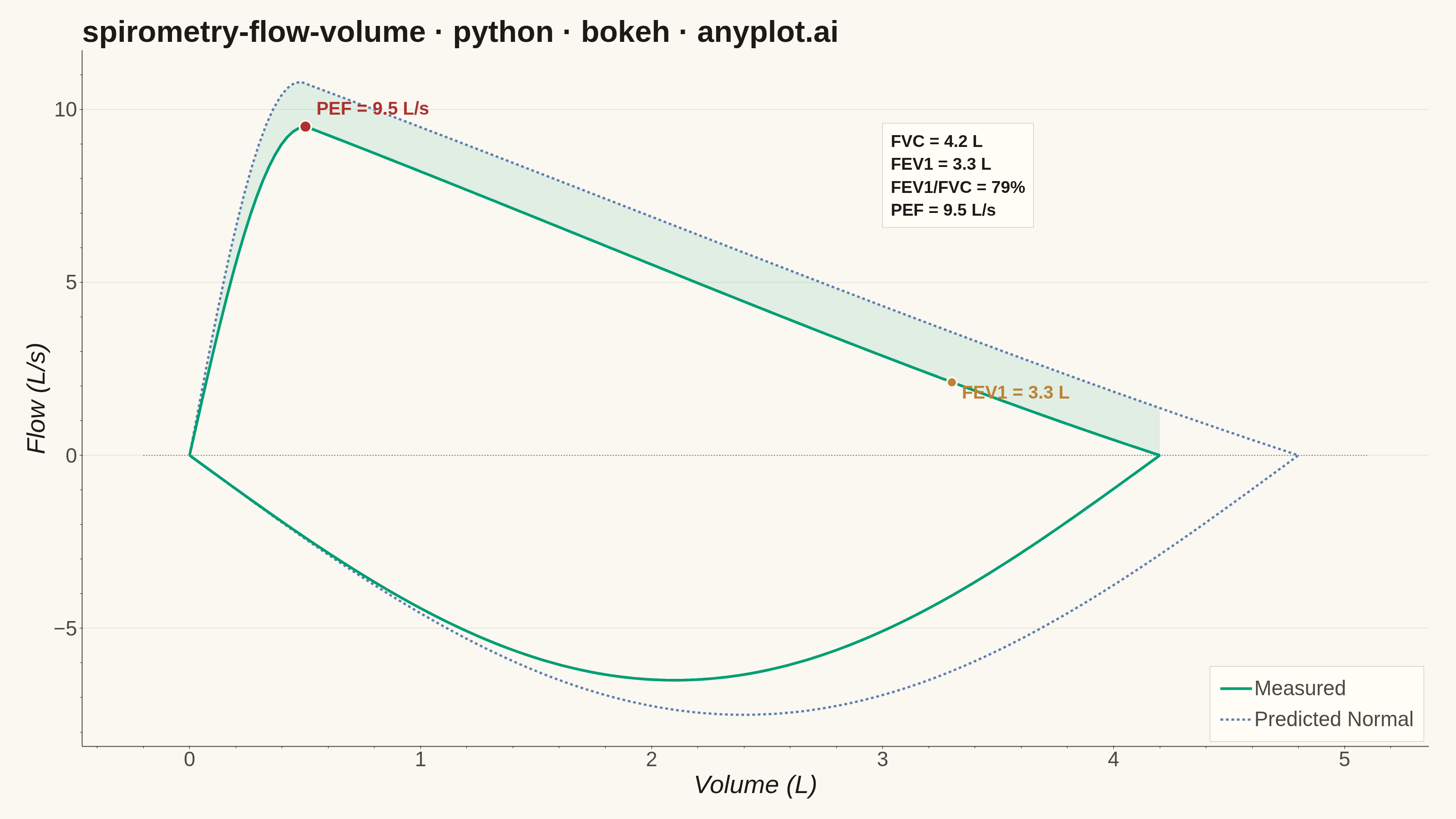
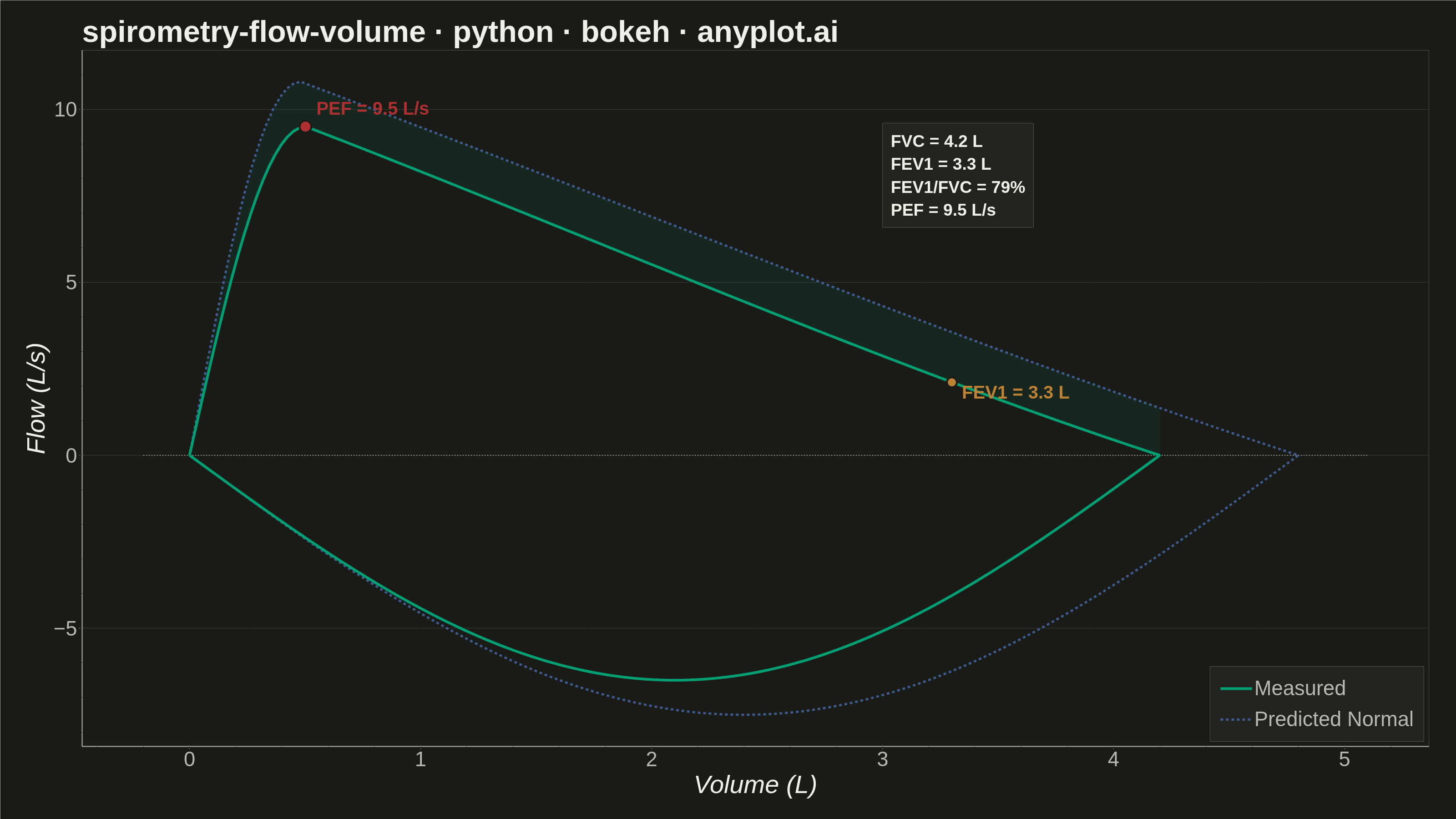
A pulmonary function test visualization that plots airflow rate (L/s) against lung volume (L) during forced expiration and inspiration, forming a characteristic loop shape. The expiratory limb rises sharply to Peak Expiratory Flow (PEF) then declines, while the inspiratory limb forms a more symmetric curve below the x-axis. This plot is essential for diagnosing obstructive and restrictive lung diseases by comparing measured loops against predicted normal values.
""" anyplot.ai
spirometry-flow-volume: Spirometry Flow-Volume Loop
Library: bokeh 3.9.1 | Python 3.13.14
Quality: 91/100 | Updated: 2026-06-17
"""

import os
import sys


# Prevent self-import: this file is named bokeh.py, which shadows the installed
# bokeh package when its directory sits at the front of sys.path.
_this_dir = os.path.dirname(os.path.abspath(__file__))
sys.path = [p for p in sys.path if os.path.abspath(p or ".") != _this_dir]

import time
from pathlib import Path

import numpy as np
from bokeh.io import output_file, save
from bokeh.models import ColumnDataSource, HoverTool, Label, Legend, LegendItem
from bokeh.plotting import figure
from selenium import webdriver
from selenium.webdriver.chrome.options import Options


# Theme tokens (see prompts/default-style-guide.md "Theme-adaptive Chrome")
THEME = os.getenv("ANYPLOT_THEME", "light")
PAGE_BG = "#FAF8F1" if THEME == "light" else "#1A1A17"
ELEVATED_BG = "#FFFDF6" if THEME == "light" else "#242420"
INK = "#1A1A17" if THEME == "light" else "#F0EFE8"
INK_SOFT = "#4A4A44" if THEME == "light" else "#B8B7B0"
INK_MUTED = "#6B6A63" if THEME == "light" else "#A8A79F"

# Imprint palette — first series ALWAYS #009E73
BRAND = "#009E73"  # measured loop (the patient)
PREDICTED = "#4467A3"  # predicted normal reference loop
ACCENT_PEF = "#AE3030"  # matte-red focal anchor for Peak Expiratory Flow
ACCENT_FEV1 = "#BD8233"  # ochre focal for FEV1 landmark

# Data — Spirometry flow-volume loop (measured vs predicted normal)
np.random.seed(42)
n_points = 160

# Clinical landmarks for a mildly-obstructed adult
fvc_measured = 4.2  # forced vital capacity (L)
pef_measured = 9.5  # peak expiratory flow (L/s)
fev1_measured = 3.3  # volume exhaled in 1 s (L)

fvc_predicted = 4.8
pef_predicted = 10.8

# Expiratory limb (measured): sharp rise to PEF then concave decline
volume_exp = np.linspace(0, fvc_measured, n_points)
t_exp = volume_exp / fvc_measured
pef_fraction = 0.12  # PEF occurs early in the forced exhalation
rise = pef_measured * np.sin(np.pi / 2 * t_exp / pef_fraction)
decline = pef_measured * (1 - (t_exp - pef_fraction) / (1 - pef_fraction))
flow_exp = np.where(t_exp <= pef_fraction, rise, decline)
flow_exp = np.maximum(flow_exp, 0.0)
flow_exp[t_exp > pef_fraction] *= 1 - 0.15 * ((t_exp[t_exp > pef_fraction] - pef_fraction) / (1 - pef_fraction)) ** 2

# Inspiratory limb (measured): symmetric U-shape below zero
volume_insp = np.linspace(fvc_measured, 0, n_points)
t_insp = np.linspace(0, 1, n_points)
peak_insp_flow = -6.5
flow_insp = peak_insp_flow * np.sin(np.pi * t_insp)

# Predicted normal — expiratory limb
volume_pred_exp = np.linspace(0, fvc_predicted, n_points)
t_pred_exp = volume_pred_exp / fvc_predicted
pef_frac_pred = 0.10
rise_pred = pef_predicted * np.sin(np.pi / 2 * t_pred_exp / pef_frac_pred)
decline_pred = pef_predicted * (1 - (t_pred_exp - pef_frac_pred) / (1 - pef_frac_pred))
flow_pred_exp = np.where(t_pred_exp <= pef_frac_pred, rise_pred, decline_pred)
flow_pred_exp = np.maximum(flow_pred_exp, 0.0)
flow_pred_exp[t_pred_exp > pef_frac_pred] *= (
    1 - 0.12 * ((t_pred_exp[t_pred_exp > pef_frac_pred] - pef_frac_pred) / (1 - pef_frac_pred)) ** 2
)

# Predicted normal — inspiratory limb
volume_pred_insp = np.linspace(fvc_predicted, 0, n_points)
peak_insp_pred = -7.5
flow_pred_insp = peak_insp_pred * np.sin(np.pi * t_insp)

# Close each loop into a single connected path
volume_measured = np.concatenate([volume_exp, volume_insp])
flow_measured = np.concatenate([flow_exp, flow_insp])
volume_predicted = np.concatenate([volume_pred_exp, volume_pred_insp])
flow_predicted = np.concatenate([flow_pred_exp, flow_pred_insp])

source_measured = ColumnDataSource(data={"volume": volume_measured, "flow": flow_measured})
source_predicted = ColumnDataSource(data={"volume": volume_predicted, "flow": flow_predicted})

# Landmark points on the measured curve
pef_idx = int(np.argmax(flow_exp))
pef_volume = volume_exp[pef_idx]
pef_flow = flow_exp[pef_idx]
fev1_idx = int(np.argmin(np.abs(volume_exp - fev1_measured)))
fev1_flow = flow_exp[fev1_idx]

# Plot
p = figure(
    width=3200,
    height=1800,
    title="spirometry-flow-volume · python · bokeh · anyplot.ai",
    x_axis_label="Volume (L)",
    y_axis_label="Flow (L/s)",
    toolbar_location=None,
    min_border_bottom=160,
    min_border_left=180,
    min_border_top=110,
    min_border_right=60,
)

# Diagnostic gap: shade between measured and predicted expiratory limbs
pred_exp_interp = np.interp(volume_exp, volume_pred_exp, flow_pred_exp)
patch_vol = np.concatenate([volume_exp, volume_exp[::-1]])
patch_flow = np.concatenate([flow_exp, pred_exp_interp[::-1]])
p.patch(x=patch_vol, y=patch_flow, fill_color=BRAND, fill_alpha=0.10, line_color=None)

# Zero-flow reference line
p.line(
    x=[-0.2, max(fvc_measured, fvc_predicted) + 0.3], y=[0, 0], line_color=INK_MUTED, line_width=2, line_dash="dotted"
)

# Predicted normal loop (dashed, background)
r_pred = p.line(
    x="volume",
    y="flow",
    source=source_predicted,
    line_color=PREDICTED,
    line_width=5,
    line_dash="dashed",
    line_alpha=0.85,
)

# Measured loop (solid, foreground)
r_meas = p.line(x="volume", y="flow", source=source_measured, line_color=BRAND, line_width=6)

# PEF focal marker + label
p.scatter(x=[pef_volume], y=[pef_flow], size=26, fill_color=ACCENT_PEF, line_color=PAGE_BG, line_width=4)
p.add_layout(
    Label(
        x=pef_volume,
        y=pef_flow,
        text=f"PEF = {pef_measured:.1f} L/s",
        text_font_size="30pt",
        text_color=ACCENT_PEF,
        text_font_style="bold",
        x_offset=24,
        y_offset=18,
    )
)

# FEV1 marker + label
p.scatter(x=[fev1_measured], y=[fev1_flow], size=22, fill_color=ACCENT_FEV1, line_color=PAGE_BG, line_width=4)
p.add_layout(
    Label(
        x=fev1_measured,
        y=fev1_flow,
        text=f"FEV1 = {fev1_measured:.1f} L",
        text_font_size="30pt",
        text_color=ACCENT_FEV1,
        text_font_style="bold",
        x_offset=22,
        y_offset=-44,
    )
)

# Clinical values box — placed in the empty upper region, clear of both limbs
clinical_text = (
    f"FVC = {fvc_measured:.1f} L\n"
    f"FEV1 = {fev1_measured:.1f} L\n"
    f"FEV1/FVC = {fev1_measured / fvc_measured:.0%}\n"
    f"PEF = {pef_measured:.1f} L/s"
)
p.add_layout(
    Label(
        x=3.0,
        y=9.6,
        text=clinical_text,
        text_font_size="28pt",
        text_color=INK,
        text_font_style="bold",
        text_baseline="top",
        background_fill_color=ELEVATED_BG,
        background_fill_alpha=0.92,
        border_line_color=INK_SOFT,
        border_line_alpha=0.35,
        padding=18,
    )
)

# Legend
legend = Legend(
    items=[LegendItem(label="Measured", renderers=[r_meas]), LegendItem(label="Predicted Normal", renderers=[r_pred])],
    location="bottom_right",
    label_text_font_size="34pt",
    label_text_color=INK_SOFT,
    glyph_width=70,
    glyph_height=34,
    spacing=16,
    padding=22,
    background_fill_color=ELEVATED_BG,
    background_fill_alpha=0.9,
    border_line_color=INK_SOFT,
    border_line_alpha=0.35,
)
p.add_layout(legend)

# Hover tool — Bokeh's interactive inspection (retained in the HTML artifact)
p.add_tools(HoverTool(tooltips=[("Volume", "@volume{0.2f} L"), ("Flow", "@flow{0.2f} L/s")], mode="mouse"))

# Style — theme-adaptive chrome
p.title.text_font_size = "50pt"
p.title.text_color = INK
p.xaxis.axis_label_text_font_size = "42pt"
p.yaxis.axis_label_text_font_size = "42pt"
p.xaxis.major_label_text_font_size = "34pt"
p.yaxis.major_label_text_font_size = "34pt"
p.xaxis.axis_label_text_color = INK
p.yaxis.axis_label_text_color = INK
p.xaxis.major_label_text_color = INK_SOFT
p.yaxis.major_label_text_color = INK_SOFT
p.xaxis.axis_line_color = INK_SOFT
p.yaxis.axis_line_color = INK_SOFT
p.xaxis.major_tick_line_color = INK_SOFT
p.yaxis.major_tick_line_color = INK_SOFT
p.xaxis.axis_line_width = 2
p.yaxis.axis_line_width = 2

# Grid — subtle y-grid only for reading flow values
p.xgrid.grid_line_color = None
p.ygrid.grid_line_color = INK
p.ygrid.grid_line_alpha = 0.15

# Backgrounds
p.background_fill_color = PAGE_BG
p.border_fill_color = PAGE_BG
p.outline_line_color = None

# Save — write interactive HTML, then screenshot via headless Chrome
output_file(f"plot-{THEME}.html")
save(p)

W, H = 3200, 1800
opts = Options()
for arg in (
    "--headless=new",
    "--no-sandbox",
    "--disable-dev-shm-usage",
    "--disable-gpu",
    f"--window-size={W},{H}",
    "--hide-scrollbars",
):
    opts.add_argument(arg)
driver = webdriver.Chrome(options=opts)
# CDP override forces an exact W×H viewport regardless of outer window chrome
driver.execute_cdp_cmd(
    "Emulation.setDeviceMetricsOverride", {"width": W, "height": H, "deviceScaleFactor": 1, "mobile": False}
)
driver.get(f"file://{Path(f'plot-{THEME}.html').resolve()}")
time.sleep(3)
driver.save_screenshot(f"plot-{THEME}.png")
driver.quit()
Runnable source as JSON, for any HTTP client: https://api.anyplot.ai/specs/spirometry-flow-volume/bokeh/code. Any spec id and library id listed in llms-full.txt fit the same URL shape; every URL below is complete and callable.
{
  "spec_id": "spirometry-flow-volume",
  "language": "python",
  "library": "bokeh",
  "page": "https://anyplot.ai/spirometry-flow-volume/python/bokeh",
  "hub": "https://anyplot.ai/spirometry-flow-volume",
  "code_json": "https://api.anyplot.ai/specs/spirometry-flow-volume/bokeh/code",
  "spec_json": "https://api.anyplot.ai/specs/spirometry-flow-volume",
  "render_light_png": "https://storage.googleapis.com/anyplot-images/plots/spirometry-flow-volume/python/bokeh/plot-light.png",
  "render_dark_png": "https://storage.googleapis.com/anyplot-images/plots/spirometry-flow-volume/python/bokeh/plot-dark.png",
  "interactive_light_html": "https://storage.googleapis.com/anyplot-images/plots/spirometry-flow-volume/python/bokeh/plot-light.html",
  "interactive_dark_html": "https://storage.googleapis.com/anyplot-images/plots/spirometry-flow-volume/python/bokeh/plot-dark.html",
  "quality_score": 91.0,
  "license": "MIT",
  "guide": "https://anyplot.ai/llms.txt"
}
Part of Spirometry Flow-Volume Loop on anyplot.ai.