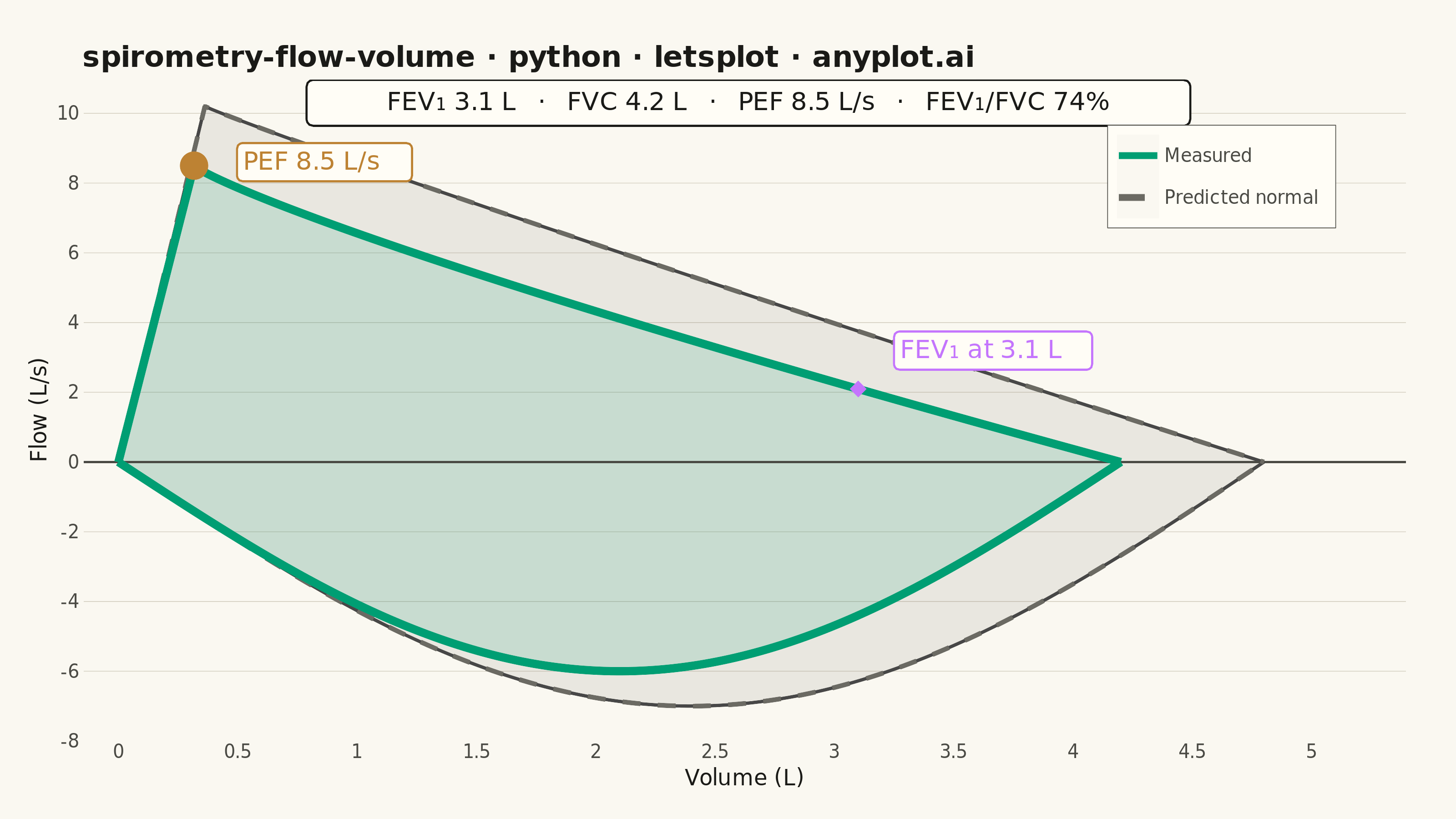
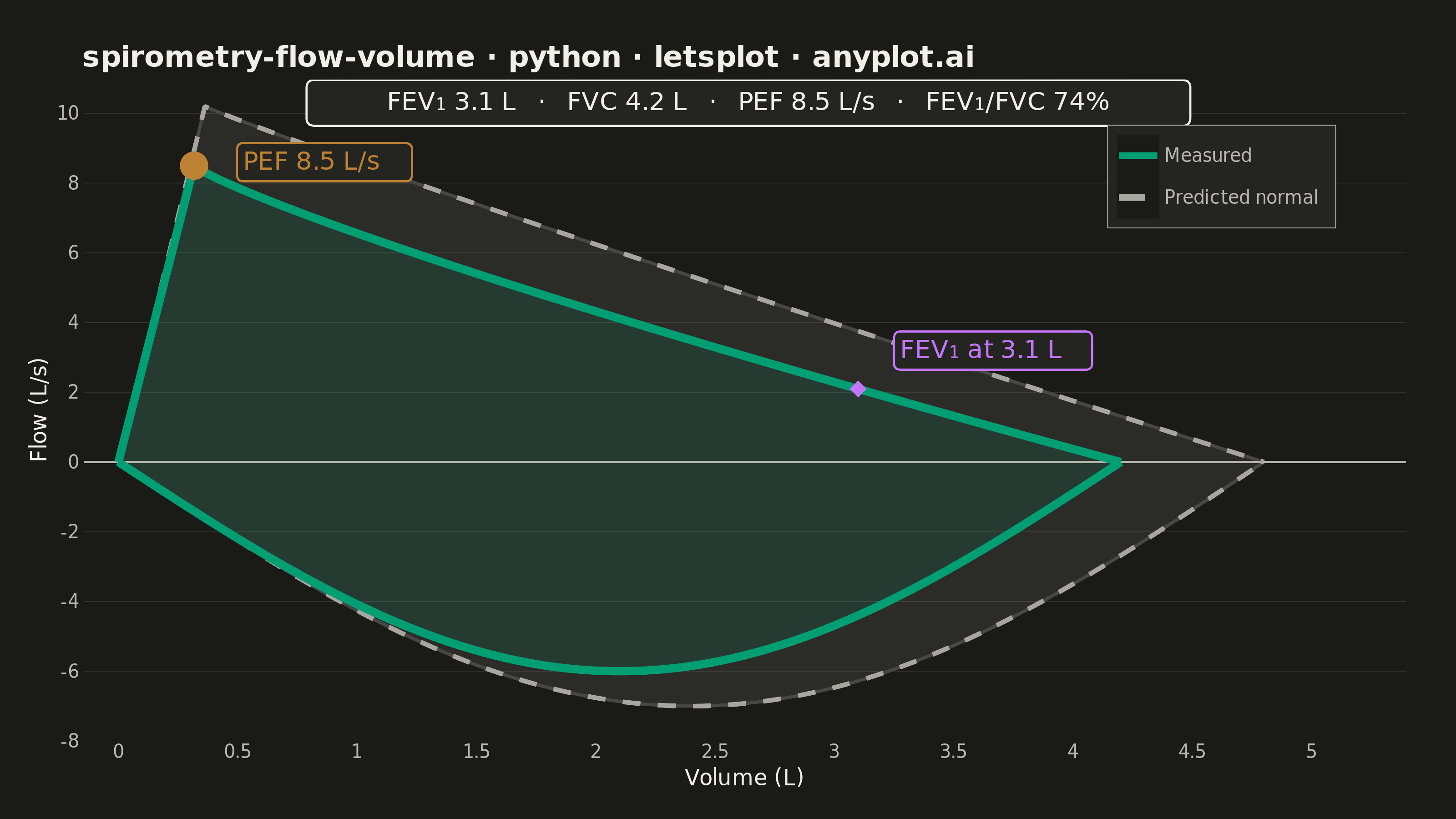
A pulmonary function test visualization that plots airflow rate (L/s) against lung volume (L) during forced expiration and inspiration, forming a characteristic loop shape. The expiratory limb rises sharply to Peak Expiratory Flow (PEF) then declines, while the inspiratory limb forms a more symmetric curve below the x-axis. This plot is essential for diagnosing obstructive and restrictive lung diseases by comparing measured loops against predicted normal values.
""" anyplot.ai
spirometry-flow-volume: Spirometry Flow-Volume Loop
Library: letsplot 4.10.1 | Python 3.13.14
Quality: 94/100 | Updated: 2026-06-17
"""

import os

import numpy as np
import pandas as pd
from lets_plot import *


LetsPlot.setup_html()

# Theme tokens (see prompts/default-style-guide.md "Theme-adaptive Chrome")
THEME = os.getenv("ANYPLOT_THEME", "light")
PAGE_BG = "#FAF8F1" if THEME == "light" else "#1A1A17"
ELEVATED_BG = "#FFFDF6" if THEME == "light" else "#242420"
INK = "#1A1A17" if THEME == "light" else "#F0EFE8"
INK_SOFT = "#4A4A44" if THEME == "light" else "#B8B7B0"
INK_MUTED = "#6B6A63" if THEME == "light" else "#A8A79F"
GRID = "#D9D4C7" if THEME == "light" else "#33322D"

# Imprint palette — data colors stay constant across themes
BRAND = "#009E73"  # measured patient loop — ALWAYS first series
PRED = INK_MUTED  # predicted normal reference (theme-adaptive muted)
PEF_COLOR = "#BD8233"  # ochre accent for Peak Expiratory Flow
FEV1_COLOR = "#C475FD"  # lavender accent for FEV1 marker

# Data: simulated spirometry flow-volume loop (mild obstructive pattern)
np.random.seed(42)

# Measured patient values
fvc = 4.2  # Forced Vital Capacity (L)
pef = 8.5  # Peak Expiratory Flow (L/s)
fev1 = 3.1  # Forced Expiratory Volume in 1 s (L)

# Expiratory limb: sharp rise to PEF then roughly linear decline
n_exp = 160
volume_exp = np.linspace(0, fvc, n_exp)
peak_idx = int(0.08 * n_exp)
flow_rise = np.linspace(0, pef, peak_idx + 1)
vol_rem = volume_exp[peak_idx:]
flow_decline = pef * (1 - ((vol_rem - vol_rem[0]) / (fvc - vol_rem[0])) ** 0.85)
flow_exp = np.concatenate([flow_rise, flow_decline[1:]])

# Inspiratory limb: symmetric U-shaped curve below the zero-flow line
n_insp = 160
volume_insp = np.linspace(fvc, 0, n_insp)
pif = -6.0  # Peak Inspiratory Flow (L/s)
flow_insp = pif * np.sin(np.linspace(0, np.pi, n_insp))

# Predicted normal values (healthy reference loop)
fvc_pred, pef_pred, pif_pred = 4.8, 10.2, -7.0
volume_pred_exp = np.linspace(0, fvc_pred, n_exp)
peak_idx_pred = int(0.08 * n_exp)
flow_pred_rise = np.linspace(0, pef_pred, peak_idx_pred + 1)
vol_rem_pred = volume_pred_exp[peak_idx_pred:]
flow_pred_decline = pef_pred * (1 - ((vol_rem_pred - vol_rem_pred[0]) / (fvc_pred - vol_rem_pred[0])) ** 0.95)
flow_pred_exp = np.concatenate([flow_pred_rise, flow_pred_decline[1:]])
volume_pred_insp = np.linspace(fvc_pred, 0, n_insp)
flow_pred_insp = pif_pred * np.sin(np.linspace(0, np.pi, n_insp))

# Curve frames (one row per limb point) with hover labels for tooltips
df_meas_exp = pd.DataFrame(
    {
        "volume": volume_exp,
        "flow": flow_exp,
        "curve": "Measured",
        "vol_label": [f"{v:.2f} L" for v in volume_exp],
        "flow_label": [f"{f:.1f} L/s" for f in flow_exp],
    }
)
df_meas_insp = pd.DataFrame(
    {
        "volume": volume_insp,
        "flow": flow_insp,
        "curve": "Measured",
        "vol_label": [f"{v:.2f} L" for v in volume_insp],
        "flow_label": [f"{f:.1f} L/s" for f in flow_insp],
    }
)
df_pred_exp = pd.DataFrame({"volume": volume_pred_exp, "flow": flow_pred_exp, "curve": "Predicted normal"})
df_pred_insp = pd.DataFrame({"volume": volume_pred_insp, "flow": flow_pred_insp, "curve": "Predicted normal"})

# Ribbon fills (loop interiors) — measured uses inspiratory limb as lower bound
df_ribbon_meas = pd.DataFrame(
    {"volume": volume_exp, "ymin": np.interp(volume_exp, volume_insp[::-1], flow_insp[::-1]), "ymax": flow_exp}
)
df_ribbon_pred = pd.DataFrame(
    {
        "volume": volume_pred_exp,
        "ymin": np.interp(volume_pred_exp, volume_pred_insp[::-1], flow_pred_insp[::-1]),
        "ymax": flow_pred_exp,
    }
)

# Clinical markers
pef_volume = volume_exp[np.argmax(flow_exp)]
df_pef = pd.DataFrame({"volume": [pef_volume], "flow": [pef]})
fev1_flow = np.interp(fev1, volume_exp, flow_exp)
df_fev1 = pd.DataFrame({"volume": [fev1], "flow": [fev1_flow]})

# Clinical summary text box (spec requires FEV1 / FVC / PEF annotations)
ratio = fev1 / fvc
clinical_text = f"FEV₁ {fev1:.1f} L   ·   FVC {fvc:.1f} L   ·   PEF {pef:.1f} L/s   ·   FEV₁/FVC {ratio:.0%}"
df_clinical = pd.DataFrame({"volume": [fvc_pred * 0.55], "flow": [10.3], "label": [clinical_text]})

title = "spirometry-flow-volume · python · letsplot · anyplot.ai"

# Plot
plot = (
    ggplot()
    # Filled loop interiors
    + geom_ribbon(aes(x="volume", ymin="ymin", ymax="ymax"), data=df_ribbon_pred, fill=PRED, alpha=0.12)
    + geom_ribbon(aes(x="volume", ymin="ymin", ymax="ymax"), data=df_ribbon_meas, fill=BRAND, alpha=0.14)
    # Zero-flow reference line dividing expiratory (upper) from inspiratory (lower)
    + geom_hline(yintercept=0, color=INK_SOFT, size=0.5)
    # Predicted normal loop (dashed) — legend driven by color + linetype aes
    + geom_line(
        aes(x="volume", y="flow", color="curve", linetype="curve"), data=df_pred_exp, size=1.1, show_legend=True
    )
    + geom_line(
        aes(x="volume", y="flow", color="curve", linetype="curve"), data=df_pred_insp, size=1.1, show_legend=False
    )
    # Measured loop (solid) with interactive tooltips
    + geom_line(
        aes(x="volume", y="flow", color="curve", linetype="curve"),
        data=df_meas_exp,
        size=2.0,
        show_legend=True,
        tooltips=layer_tooltips().title("Expiratory limb").line("Volume|@vol_label").line("Flow|@flow_label"),
    )
    + geom_line(
        aes(x="volume", y="flow", color="curve", linetype="curve"),
        data=df_meas_insp,
        size=2.0,
        show_legend=False,
        tooltips=layer_tooltips().title("Inspiratory limb").line("Volume|@vol_label").line("Flow|@flow_label"),
    )
    # FEV1 marker
    + geom_point(aes(x="volume", y="flow"), data=df_fev1, color=FEV1_COLOR, size=6, shape=18)
    + geom_label(
        aes(x="volume", y="flow", label="label"),
        data=pd.DataFrame({"volume": [fev1 + 0.15], "flow": [fev1_flow + 1.1], "label": [f"FEV₁ at {fev1:.1f} L"]}),
        size=7,
        color=FEV1_COLOR,
        fill=ELEVATED_BG,
        label_padding=0.25,
        hjust=0,
    )
    # PEF marker
    + geom_point(
        aes(x="volume", y="flow"),
        data=df_pef,
        color=PEF_COLOR,
        size=7,
        shape=16,
        tooltips=layer_tooltips()
        .title("Peak Expiratory Flow")
        .line(f"PEF|{pef} L/s")
        .line(f"Volume|{pef_volume:.2f} L"),
    )
    + geom_label(
        aes(x="volume", y="flow", label="label"),
        data=pd.DataFrame({"volume": [pef_volume + 0.18], "flow": [pef + 0.1], "label": [f"PEF {pef} L/s"]}),
        size=7,
        color=PEF_COLOR,
        fill=ELEVATED_BG,
        label_padding=0.25,
        hjust=0,
    )
    # Clinical summary
    + geom_label(
        aes(x="volume", y="flow", label="label"),
        data=df_clinical,
        size=7,
        color=INK,
        fill=ELEVATED_BG,
        label_padding=0.4,
        hjust=0.5,
    )
    # Scales — combined color + linetype legend (shared empty name merges them)
    + scale_color_manual(values={"Measured": BRAND, "Predicted normal": PRED}, name="")
    + scale_linetype_manual(values={"Measured": "solid", "Predicted normal": "dashed"}, name="")
    + guides(color=guide_legend(override_aes={"size": 1.6}))
    + labs(x="Volume (L)", y="Flow (L/s)", title=title)
    + coord_cartesian(xlim=[-0.15, 5.4], ylim=[-8, 11])
    + scale_y_continuous(breaks=list(range(-8, 12, 2)))
    # Sizing & theme-adaptive chrome
    + ggsize(800, 450)
    + theme_minimal()
    + theme(
        plot_title=element_text(size=16, face="bold", color=INK),
        axis_title=element_text(size=12, color=INK),
        axis_text=element_text(size=10, color=INK_SOFT),
        panel_grid_major_y=element_line(color=GRID, size=0.4),
        panel_grid_major_x=element_blank(),
        panel_grid_minor=element_blank(),
        panel_border=element_blank(),
        axis_line=element_blank(),
        axis_ticks=element_blank(),
        legend_position=[0.86, 0.93],
        legend_justification=[0.5, 1.0],
        legend_text=element_text(size=10, color=INK_SOFT),
        legend_background=element_rect(fill=ELEVATED_BG, color=INK_SOFT, size=0.4),
        plot_background=element_rect(fill=PAGE_BG, color=PAGE_BG),
        panel_background=element_rect(fill=PAGE_BG, color=PAGE_BG),
        plot_margin=[24, 24, 16, 16],
    )
)

# Save
ggsave(plot, f"plot-{THEME}.png", scale=4, path=".")
ggsave(plot, f"plot-{THEME}.html", path=".")
Runnable source as JSON, for any HTTP client: https://api.anyplot.ai/specs/spirometry-flow-volume/letsplot/code. Any spec id and library id listed in llms-full.txt fit the same URL shape; every URL below is complete and callable.
{
  "spec_id": "spirometry-flow-volume",
  "language": "python",
  "library": "letsplot",
  "page": "https://anyplot.ai/spirometry-flow-volume/python/letsplot",
  "hub": "https://anyplot.ai/spirometry-flow-volume",
  "code_json": "https://api.anyplot.ai/specs/spirometry-flow-volume/letsplot/code",
  "spec_json": "https://api.anyplot.ai/specs/spirometry-flow-volume",
  "render_light_png": "https://storage.googleapis.com/anyplot-images/plots/spirometry-flow-volume/python/letsplot/plot-light.png",
  "render_dark_png": "https://storage.googleapis.com/anyplot-images/plots/spirometry-flow-volume/python/letsplot/plot-dark.png",
  "interactive_light_html": "https://storage.googleapis.com/anyplot-images/plots/spirometry-flow-volume/python/letsplot/plot-light.html",
  "interactive_dark_html": "https://storage.googleapis.com/anyplot-images/plots/spirometry-flow-volume/python/letsplot/plot-dark.html",
  "quality_score": 94.0,
  "license": "MIT",
  "guide": "https://anyplot.ai/llms.txt"
}
Part of Spirometry Flow-Volume Loop on anyplot.ai.