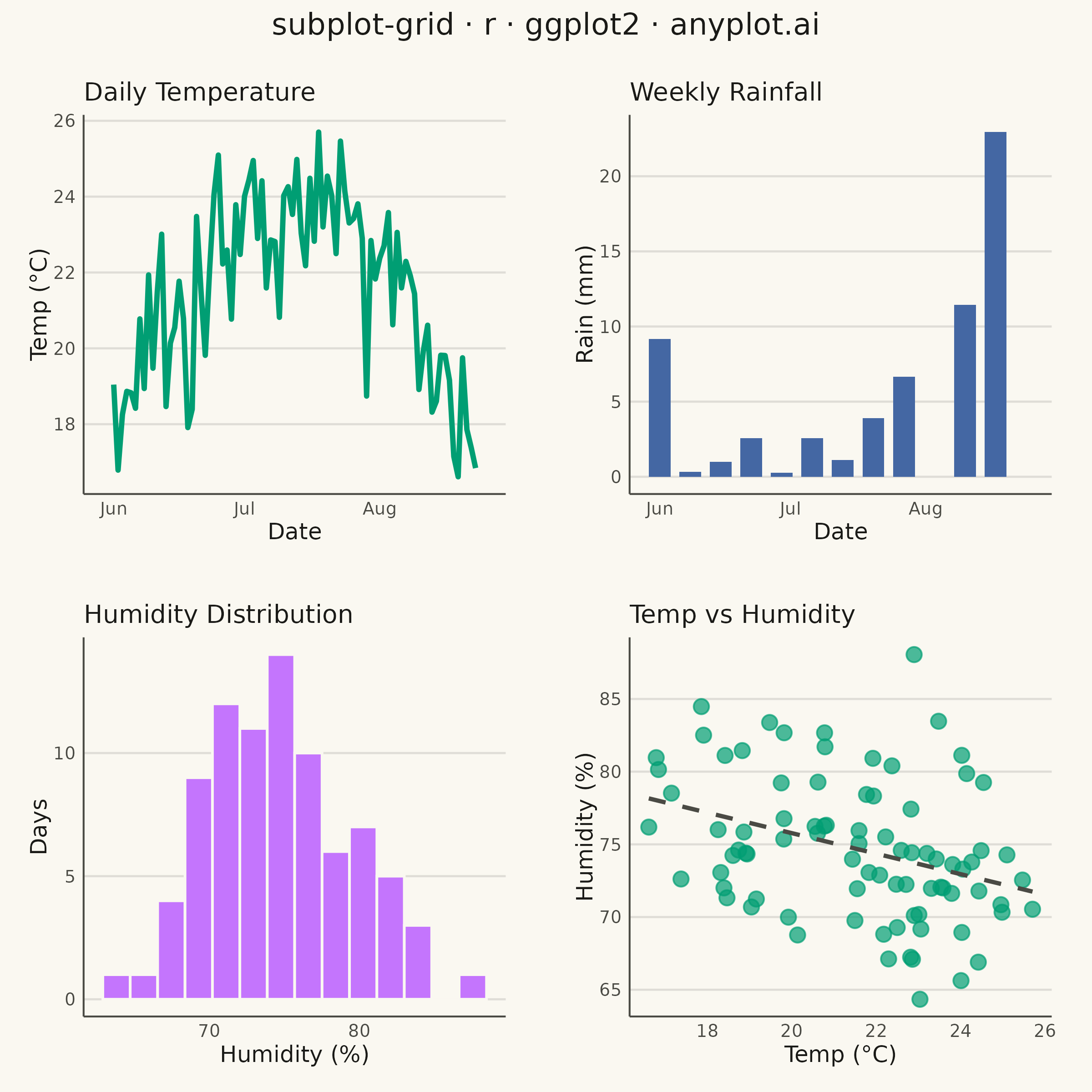
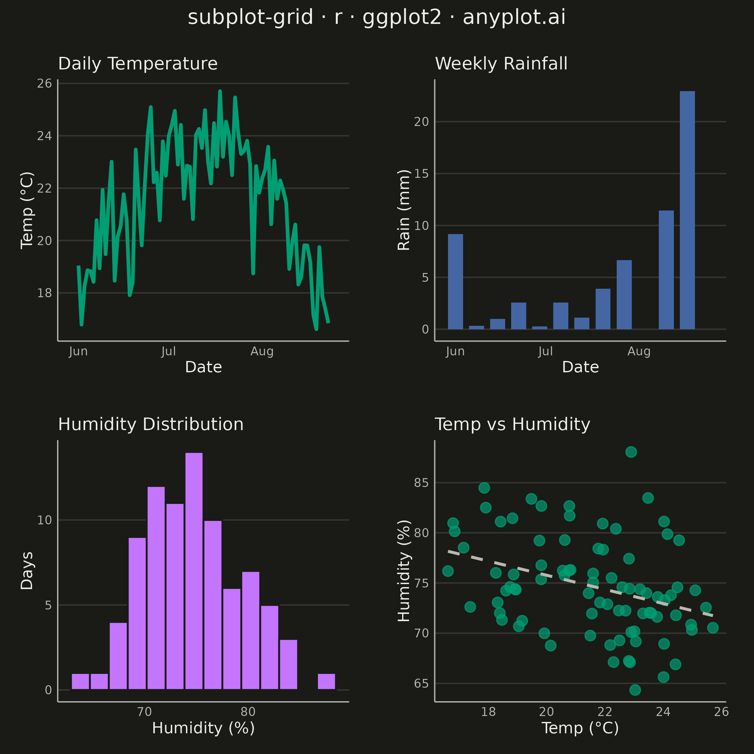
The same plot in 14 other libraries — Python: Altair, Bokeh, lets-plot, Matplotlib, Plotly, plotnine, Pygal, Seaborn; Julia: Makie.jl; JavaScript: Chart.js, D3.js, Apache ECharts, Highcharts, MUI X Charts. Compare all 15 side by side: Subplot Grid Layout in Python, R, Julia and JavaScript.
A customizable grid of multiple subplots allowing different plot types in each cell, with shared or independent axes. Unlike faceted plots that repeat the same visualization for data subsets, subplot grids enable combining distinct visualizations (scatter, line, bar, histogram, etc.) into a cohesive multi-panel figure for comprehensive data presentation.
#' anyplot.ai
#' subplot-grid: Subplot Grid Layout
#' Library: ggplot2 3.5.1 | R 4.4.1
#' Quality: 88/100 | Created: 2026-09-09

library(ggplot2)
library(dplyr)
library(scales)
library(ragg)
library(gridExtra)

grDevices::pdf(NULL)  # null device so building text grobs pre-render doesn't leave a stray Rplots.pdf
set.seed(42)

# --- Theme tokens ------------------------------------------------------
THEME    <- Sys.getenv("ANYPLOT_THEME", "light")
PAGE_BG  <- if (THEME == "light") "#FAF8F1" else "#1A1A17"
INK      <- if (THEME == "light") "#1A1A17" else "#F0EFE8"
INK_SOFT <- if (THEME == "light") "#4A4A44" else "#B8B7B0"

IMPRINT_PALETTE <- c("#009E73", "#C475FD", "#4467A3", "#BD8233",
                     "#AE3030", "#2ABCCD", "#954477", "#99B314")

# --- Data: a 12-week weather-station log combining four complementary ------
# views of the same station (daily temperature, weekly rainfall totals,
# humidity distribution, temperature-humidity relationship) — the point of a
# subplot grid is mixing distinct plot types, not repeating one geom.
n_days <- 84
dates  <- seq(as.Date("2024-06-01"), by = "day", length.out = n_days)
day_idx <- seq_len(n_days)

temp_c <- 17 + 7 * sin(pi * day_idx / n_days) + rnorm(n_days, mean = 0, sd = 1.3)
humidity_pct <- 78 - 0.55 * (temp_c - min(temp_c)) + rnorm(n_days, mean = 0, sd = 5)
humidity_pct <- pmin(pmax(humidity_pct, 25), 95)
precip_mm <- rgamma(n_days, shape = 0.35, scale = 6) * rbinom(n_days, 1, 0.4)

station <- tibble::tibble(
  date         = dates,
  week         = ((day_idx - 1) %/% 7) + 1,
  temp_c       = temp_c,
  humidity_pct = humidity_pct,
  precip_mm    = precip_mm
)

weekly_precip <- station %>%
  group_by(week) %>%
  summarise(total_precip_mm = sum(precip_mm), week_start = min(date), .groups = "drop")

# Shared x-axis range (date) for the top row: temperature and rainfall come
# from the same 12-week station log, so aligning them on one time axis lets
# the two panels be compared directly -- the spec's "shared axes" mode,
# alongside the independent y-scales used by every other panel. Padded by
# half the rainfall bar width so the first/last bars aren't clipped by the
# shared limits.
date_range <- range(station$date) + c(-2.5, 2.5)

# --- Title ---------------------------------------------------------------
title_text <- "subplot-grid · r · ggplot2 · anyplot.ai"
title_fontsize <- if (nchar(title_text) > 67) round(12 * 67 / nchar(title_text)) else 12
title_fontsize <- max(title_fontsize, 8)
FONT_FAMILY <- "sans"

# --- Shared chrome ---------------------------------------------------------
anyplot_theme <- theme_minimal(base_size = 7, base_family = FONT_FAMILY) +
  theme(
    plot.background     = element_rect(fill = PAGE_BG, color = PAGE_BG),
    panel.background    = element_rect(fill = PAGE_BG, color = NA),
    panel.grid.minor    = element_blank(),
    panel.grid.major.x  = element_blank(),
    panel.grid.major.y  = element_line(color = alpha(INK, 0.12), linewidth = 0.4),
    axis.line           = element_line(color = INK_SOFT, linewidth = 0.35),
    axis.ticks          = element_blank(),
    axis.title          = element_text(color = INK, size = 9),
    axis.text           = element_text(color = INK_SOFT, size = 7),
    plot.title          = element_text(color = INK, size = 10, face = "plain"),
    plot.margin         = margin(t = 14, r = 16, b = 10, l = 12)
  )

# --- Panel 1: daily temperature (line) -- shared date axis with panel 2 ----
p_temp <- ggplot(station, aes(x = date, y = temp_c)) +
  geom_line(color = IMPRINT_PALETTE[1], linewidth = 1.0) +
  scale_x_date(limits = date_range, date_labels = "%b") +
  labs(title = "Daily Temperature", x = "Date", y = "Temp (°C)") +
  anyplot_theme

# --- Panel 2: weekly rainfall (bar) -- shared date axis with panel 1 ------
# blue for the water association; x uses the same date range/scale as panel 1
# so the two time series line up for direct visual comparison.
p_precip <- ggplot(weekly_precip, aes(x = week_start, y = total_precip_mm)) +
  geom_col(fill = IMPRINT_PALETTE[3], width = 5) +
  scale_x_date(limits = date_range, date_labels = "%b") +
  labs(title = "Weekly Rainfall", x = "Date", y = "Rain (mm)") +
  anyplot_theme

# --- Panel 3: humidity distribution (histogram) -----------------------------
p_humidity <- ggplot(station, aes(x = humidity_pct)) +
  geom_histogram(fill = IMPRINT_PALETTE[2], color = PAGE_BG, bins = 14) +
  labs(title = "Humidity Distribution", x = "Humidity (%)", y = "Days") +
  anyplot_theme

# --- Panel 4: temperature vs humidity (scatter) -----------------------------
p_scatter <- ggplot(station, aes(x = temp_c, y = humidity_pct)) +
  geom_point(color = IMPRINT_PALETTE[1], size = 2.5, alpha = 0.7) +
  geom_smooth(method = "lm", formula = y ~ x, se = FALSE,
              color = INK_SOFT, linewidth = 0.8, linetype = "dashed") +
  labs(title = "Temp vs Humidity", x = "Temp (°C)", y = "Humidity (%)") +
  anyplot_theme

# --- Combine into a 2x2 grid with a shared anyplot title ---------------------
combined <- arrangeGrob(
  p_temp, p_precip, p_humidity, p_scatter,
  ncol = 2, nrow = 2,
  top = grid::textGrob(
    title_text,
    gp = grid::gpar(col = INK, fontsize = title_fontsize, fontfamily = FONT_FAMILY)
  ),
  padding = grid::unit(10, "pt")
)

# --- Save --------------------------------------------------------------------
ggsave(
  filename = sprintf("plot-%s.png", THEME),
  plot     = combined,
  device   = ragg::agg_png,
  width    = 6,
  height   = 6,
  units    = "in",
  dpi      = 400,
  bg       = PAGE_BG
)
Runnable source as JSON, for any HTTP client: https://api.anyplot.ai/specs/subplot-grid/ggplot2/code. Any spec id and library id listed in llms-full.txt fit the same URL shape; every URL below is complete and callable.
{
  "spec_id": "subplot-grid",
  "language": "r",
  "library": "ggplot2",
  "page": "https://anyplot.ai/subplot-grid/r/ggplot2",
  "hub": "https://anyplot.ai/subplot-grid",
  "code_json": "https://api.anyplot.ai/specs/subplot-grid/ggplot2/code",
  "spec_json": "https://api.anyplot.ai/specs/subplot-grid",
  "render_light_png": "https://storage.googleapis.com/anyplot-images/plots/subplot-grid/r/ggplot2/plot-light.png",
  "render_dark_png": "https://storage.googleapis.com/anyplot-images/plots/subplot-grid/r/ggplot2/plot-dark.png",
  "quality_score": 88.0,
  "license": "MIT",
  "guide": "https://anyplot.ai/llms.txt"
}
Part of Subplot Grid Layout on anyplot.ai.