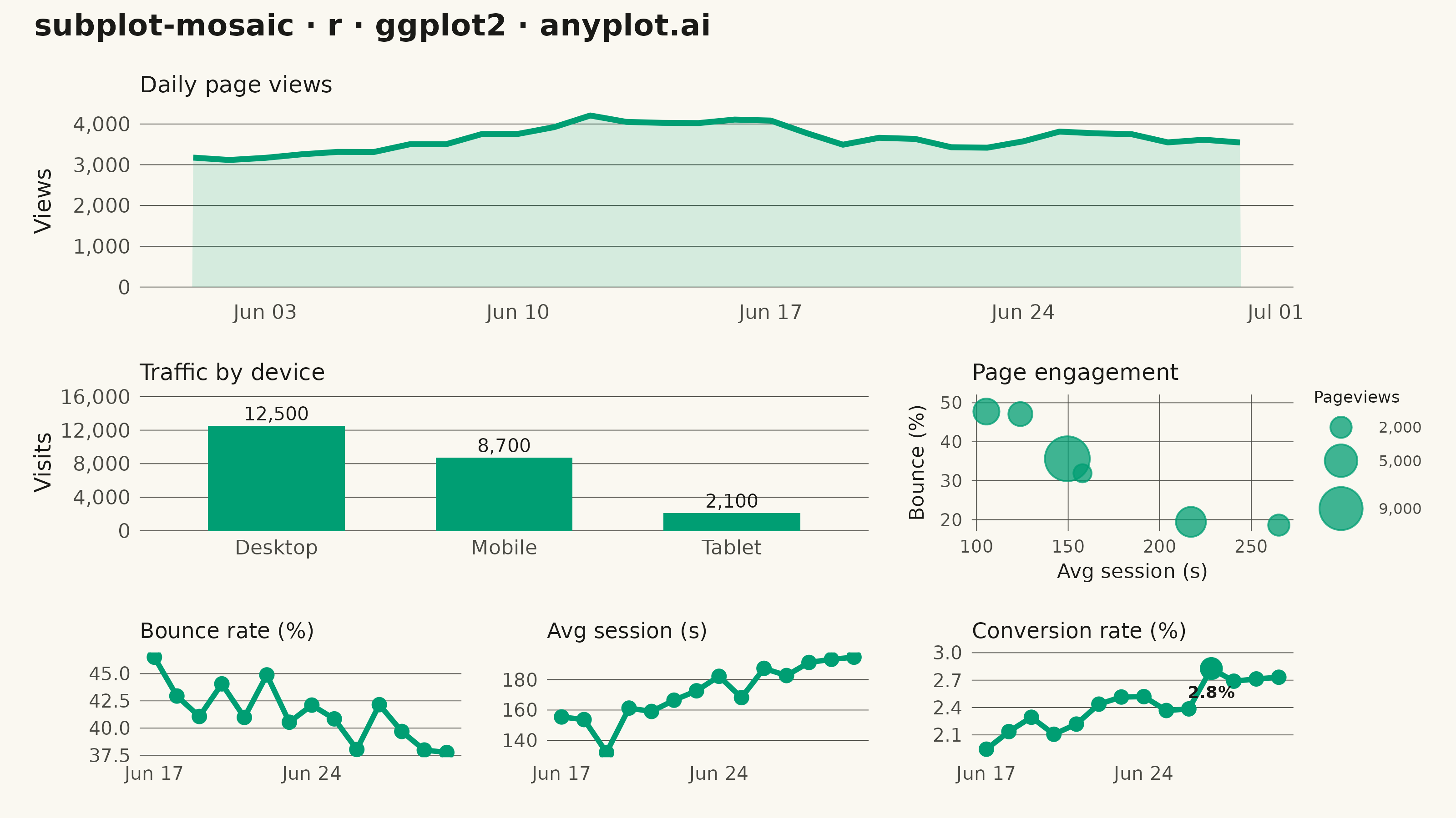
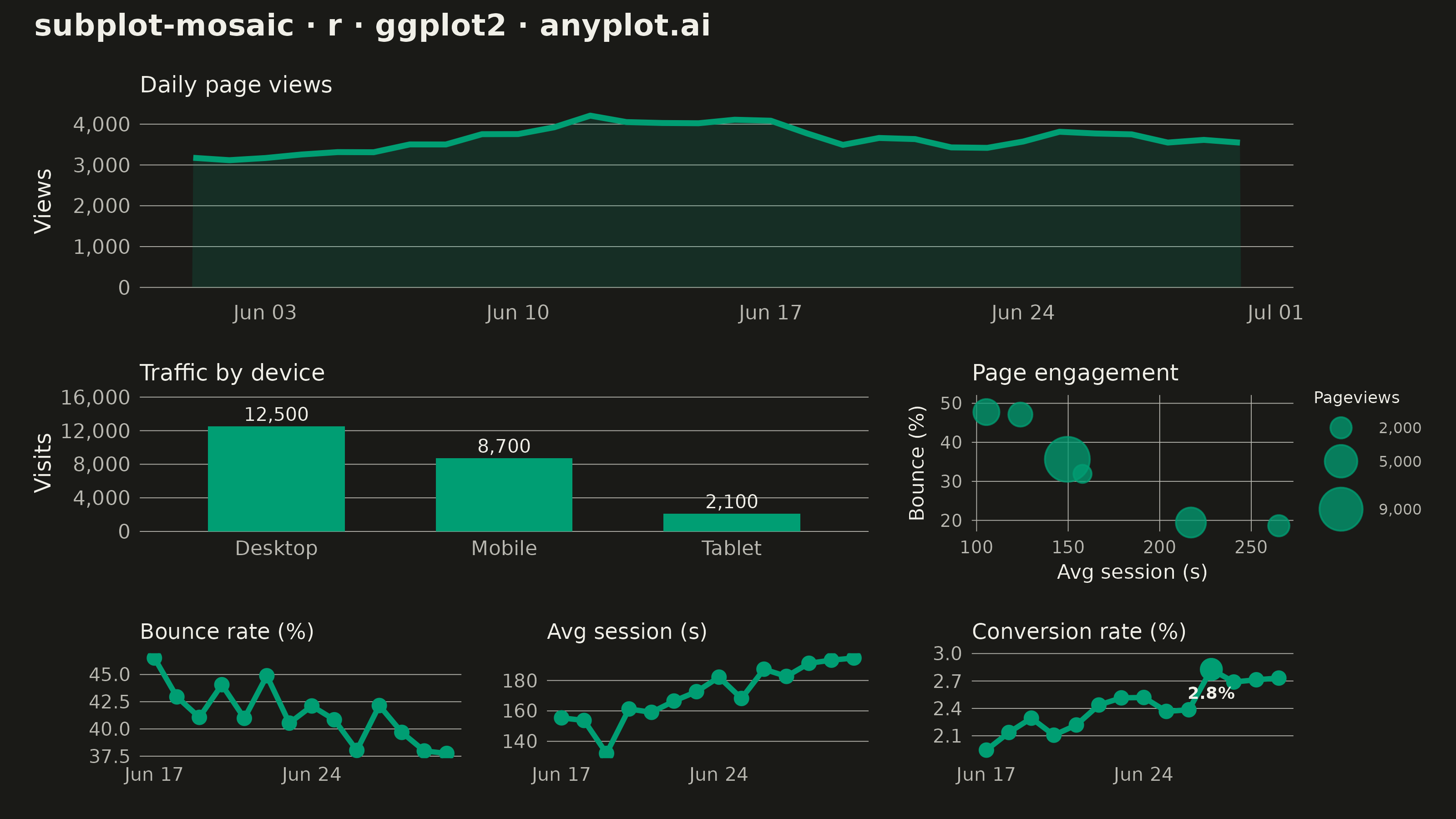
The same plot in 14 other libraries — Python: Altair, Bokeh, lets-plot, Matplotlib, Plotly, plotnine, Pygal, Seaborn; Julia: Makie.jl; JavaScript: Chart.js, D3.js, Apache ECharts, Highcharts, MUI X Charts. Compare all 15 side by side: Mosaic Subplot Layout with Varying Sizes in Python, R, Julia and JavaScript.
A complex subplot layout where different subplots can have varying sizes and arrangements using intuitive ASCII-art style string definitions. Unlike GridSpec approaches that require explicit row/column spanning, mosaic layouts allow defining layouts through visual string patterns (e.g., "AB;CC" creates A and B on top, C spanning below), making complex configurations more readable and maintainable.
#' anyplot.ai
#' subplot-mosaic: Mosaic Subplot Layout with Varying Sizes
#' Library: ggplot2 3.5.1 | R 4.4.1
#' Quality: 88/100 | Created: 2026-09-09

library(ggplot2)
library(patchwork)
library(ragg)

set.seed(42)

# --- Theme tokens ------------------------------------------------------------
THEME       <- Sys.getenv("ANYPLOT_THEME", "light")
PAGE_BG     <- if (THEME == "light") "#FAF8F1" else "#1A1A17"
INK         <- if (THEME == "light") "#1A1A17" else "#F0EFE8"
INK_SOFT    <- if (THEME == "light") "#4A4A44" else "#B8B7B0"
IMPRINT_PALETTE <- c("#009E73", "#C475FD", "#4467A3", "#BD8233",
                     "#AE3030", "#2ABCCD", "#954477", "#99B314")
BRAND <- IMPRINT_PALETTE[1]

# --- Data ----------------------------------------------------------------
# Website analytics dashboard, mosaic layout "AAA;BBC;DEF"
dates <- seq(as.Date("2024-06-01"), by = "day", length.out = 30)
page_views <- pmax(500, round(3000 + cumsum(rnorm(30, mean = 10, sd = 120))))
overview_df <- data.frame(date = dates, page_views = page_views)

devices <- factor(c("Desktop", "Mobile", "Tablet"), levels = c("Desktop", "Mobile", "Tablet"))
device_visits <- c(12500, 8700, 2100)
device_df <- data.frame(device = devices, visits = device_visits)

pages <- c("Home", "Blog", "Product", "Pricing", "Docs", "Support")
avg_session_sec <- c(145, 210, 95, 130, 260, 175) + rnorm(6, 0, 10)
bounce_rate_pct <- c(38, 22, 55, 47, 18, 33) + rnorm(6, 0, 3)
page_pageviews <- c(9800, 4200, 3100, 2600, 2000, 1400)
pages_df <- data.frame(
  page = pages,
  avg_session_sec = avg_session_sec,
  bounce_rate_pct = bounce_rate_pct,
  pageviews = page_pageviews
)

recent_days <- dates[17:30]
bounce_trend <- pmax(10, 45 - seq(0, 13) * 0.6 + rnorm(14, 0, 2))
session_trend <- 150 + seq(0, 13) * 3 + rnorm(14, 0, 8)
conversion_trend <- pmax(0, 2.1 + seq(0, 13) * 0.05 + rnorm(14, 0, 0.15))
bounce_df <- data.frame(date = recent_days, value = bounce_trend)
session_df <- data.frame(date = recent_days, value = session_trend)
conversion_df <- data.frame(date = recent_days, value = conversion_trend)

# --- Shared chrome -----------------------------------------------------------
base_chrome <- theme_minimal(base_size = 8) +
  theme(
    plot.background   = element_rect(fill = PAGE_BG, color = PAGE_BG),
    panel.background  = element_rect(fill = PAGE_BG, color = NA),
    panel.grid.minor  = element_blank(),
    panel.grid.major  = element_line(color = INK_SOFT, linewidth = 0.15),
    axis.title        = element_text(color = INK),
    axis.text         = element_text(color = INK_SOFT),
    plot.title        = element_text(color = INK, face = "plain", size = 9, hjust = 0),
    legend.position   = "none",
    plot.margin       = margin(8, 8, 8, 8, unit = "pt")
  )

# --- Panel A: overview (wide, top row) ---------------------------------------
panel_a <- ggplot(overview_df, aes(date, page_views)) +
  geom_area(fill = BRAND, alpha = 0.15) +
  geom_line(color = BRAND, linewidth = 1.1) +
  labs(title = "Daily page views", x = NULL, y = "Views") +
  scale_y_continuous(labels = scales::comma) +
  base_chrome +
  theme(
    panel.grid.major.x = element_blank(),
    axis.title.y = element_text(size = 9), axis.text = element_text(size = 8)
  )

# --- Panel B: device breakdown (medium, spans 2 cols) -------------------------
panel_b <- ggplot(device_df, aes(device, visits)) +
  geom_col(fill = BRAND, width = 0.6) +
  geom_text(
    aes(label = scales::comma(visits)), vjust = -0.4, size = 2.6, color = INK
  ) +
  labs(title = "Traffic by device", x = NULL, y = "Visits") +
  scale_y_continuous(labels = scales::comma, expand = expansion(mult = c(0, 0.3))) +
  coord_cartesian(clip = "off") +
  base_chrome +
  theme(
    panel.grid.major.x = element_blank(),
    axis.title.y = element_text(size = 9), axis.text = element_text(size = 8)
  )

# --- Panel C: page engagement (medium) ----------------------------------------
panel_c <- ggplot(pages_df, aes(avg_session_sec, bounce_rate_pct)) +
  geom_point(aes(size = pageviews), color = BRAND, alpha = 0.75) +
  labs(title = "Page engagement", x = "Avg session (s)", y = "Bounce (%)") +
  scale_size_area(
    name = "Pageviews", max_size = 8,
    breaks = c(2000, 5000, 9000), labels = scales::comma
  ) +
  scale_y_continuous(expand = expansion(mult = c(0.05, 0.15))) +
  coord_cartesian(clip = "off") +
  base_chrome +
  theme(
    axis.title         = element_text(size = 8),
    axis.text          = element_text(size = 7),
    legend.position    = "right",
    legend.background  = element_rect(fill = PAGE_BG, color = NA),
    legend.text        = element_text(size = 6, color = INK_SOFT),
    legend.title        = element_text(size = 6.5, color = INK),
    legend.key.size     = unit(8, "pt"),
    legend.margin       = margin(0, 0, 0, 0)
  )

# --- Panels D/E/F: small metric trends (bottom row) ---------------------------
small_chrome <- base_chrome +
  theme(
    panel.grid.major.x = element_blank(),
    axis.title  = element_blank(),
    axis.text.y = element_text(size = 7.5),
    axis.text.x = element_text(size = 7.5),
    plot.title  = element_text(size = 8.5)
  )

peak_label <- function(df) {
  df[which.max(df$value), , drop = FALSE]
}

panel_d <- ggplot(bounce_df, aes(date, value)) +
  geom_line(color = BRAND, linewidth = 1.0) +
  geom_point(color = BRAND, size = 2.2) +
  labs(title = "Bounce rate (%)") +
  small_chrome

panel_e <- ggplot(session_df, aes(date, value)) +
  geom_line(color = BRAND, linewidth = 1.0) +
  geom_point(color = BRAND, size = 2.2) +
  labs(title = "Avg session (s)") +
  small_chrome

conversion_peak <- peak_label(conversion_df)
panel_f <- ggplot(conversion_df, aes(date, value)) +
  geom_line(color = BRAND, linewidth = 1.0) +
  geom_point(color = BRAND, size = 2.2) +
  geom_point(data = conversion_peak, color = BRAND, size = 3.6) +
  geom_text(
    data = conversion_peak, aes(label = sprintf("%.1f%%", value)),
    vjust = 2.4, size = 2.4, color = INK, fontface = "bold"
  ) +
  labs(title = "Conversion rate (%)") +
  scale_y_continuous(expand = expansion(mult = c(0.1, 0.2))) +
  coord_cartesian(clip = "off") +
  small_chrome

# --- Mosaic assembly -----------------------------------------------------
# Layout string:  "AAA
#                  BBC
#                  DEF"
# patchwork::wrap_plots() composites full plot grobs (including each panel's
# own legend, and any coord_cartesian(clip = "off") overflow) instead of
# gridExtra::arrangeGrob(), which drops per-panel legends and re-clips
# overflow at each fixed grid-cell boundary.
title_text <- "subplot-mosaic · r · ggplot2 · anyplot.ai"

mosaic <- wrap_plots(
  A = panel_a, B = panel_b, C = panel_c,
  D = panel_d, E = panel_e, F = panel_f,
  design = "AAA\nBBC\nDEF",
  heights = c(1.8, 1.3, 1)
) +
  plot_annotation(
    title = title_text,
    theme = theme(
      plot.title      = element_text(size = 12, face = "bold", color = INK, hjust = 0),
      plot.background = element_rect(fill = PAGE_BG, color = PAGE_BG)
    )
  )

# --- Save ----------------------------------------------------------------
ggsave(
  filename = sprintf("plot-%s.png", THEME),
  plot     = mosaic,
  device   = ragg::agg_png,
  width    = 8,
  height   = 4.5,
  units    = "in",
  dpi      = 400,
  bg       = PAGE_BG
)
Runnable source as JSON, for any HTTP client: https://api.anyplot.ai/specs/subplot-mosaic/ggplot2/code. Any spec id and library id listed in llms-full.txt fit the same URL shape; every URL below is complete and callable.
{
  "spec_id": "subplot-mosaic",
  "language": "r",
  "library": "ggplot2",
  "page": "https://anyplot.ai/subplot-mosaic/r/ggplot2",
  "hub": "https://anyplot.ai/subplot-mosaic",
  "code_json": "https://api.anyplot.ai/specs/subplot-mosaic/ggplot2/code",
  "spec_json": "https://api.anyplot.ai/specs/subplot-mosaic",
  "render_light_png": "https://storage.googleapis.com/anyplot-images/plots/subplot-mosaic/r/ggplot2/plot-light.png",
  "render_dark_png": "https://storage.googleapis.com/anyplot-images/plots/subplot-mosaic/r/ggplot2/plot-dark.png",
  "quality_score": 88.0,
  "license": "MIT",
  "guide": "https://anyplot.ai/llms.txt"
}
Part of Mosaic Subplot Layout with Varying Sizes on anyplot.ai.