The same plot in 14 other libraries — JavaScript: Chart.js, Apache ECharts, Highcharts, MUI X Charts; Python: Altair, Bokeh, lets-plot, Matplotlib, Plotly, plotnine, Pygal, Seaborn; R: ggplot2; Julia: Makie.jl. Compare all 15 side by side: Acid-Base Titration Curve in Python, R, Julia and JavaScript.
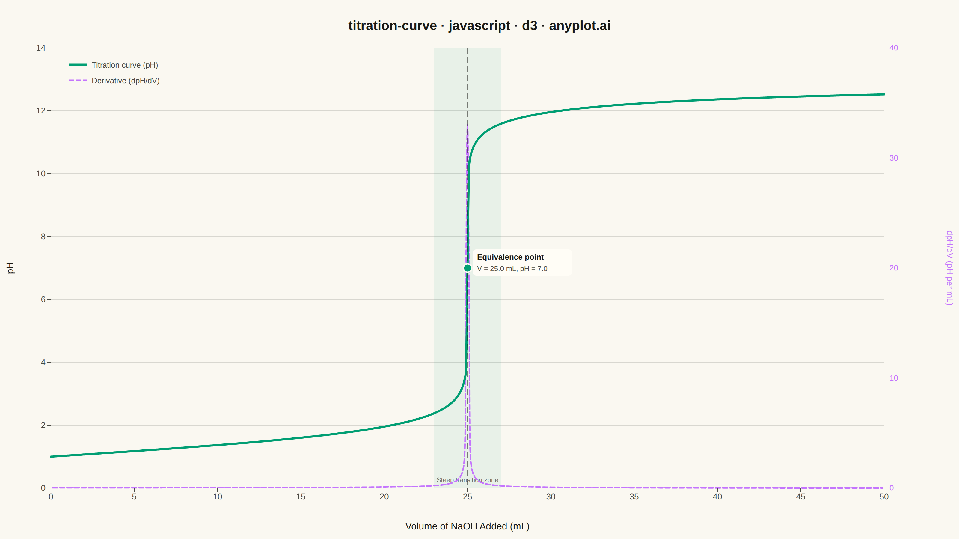
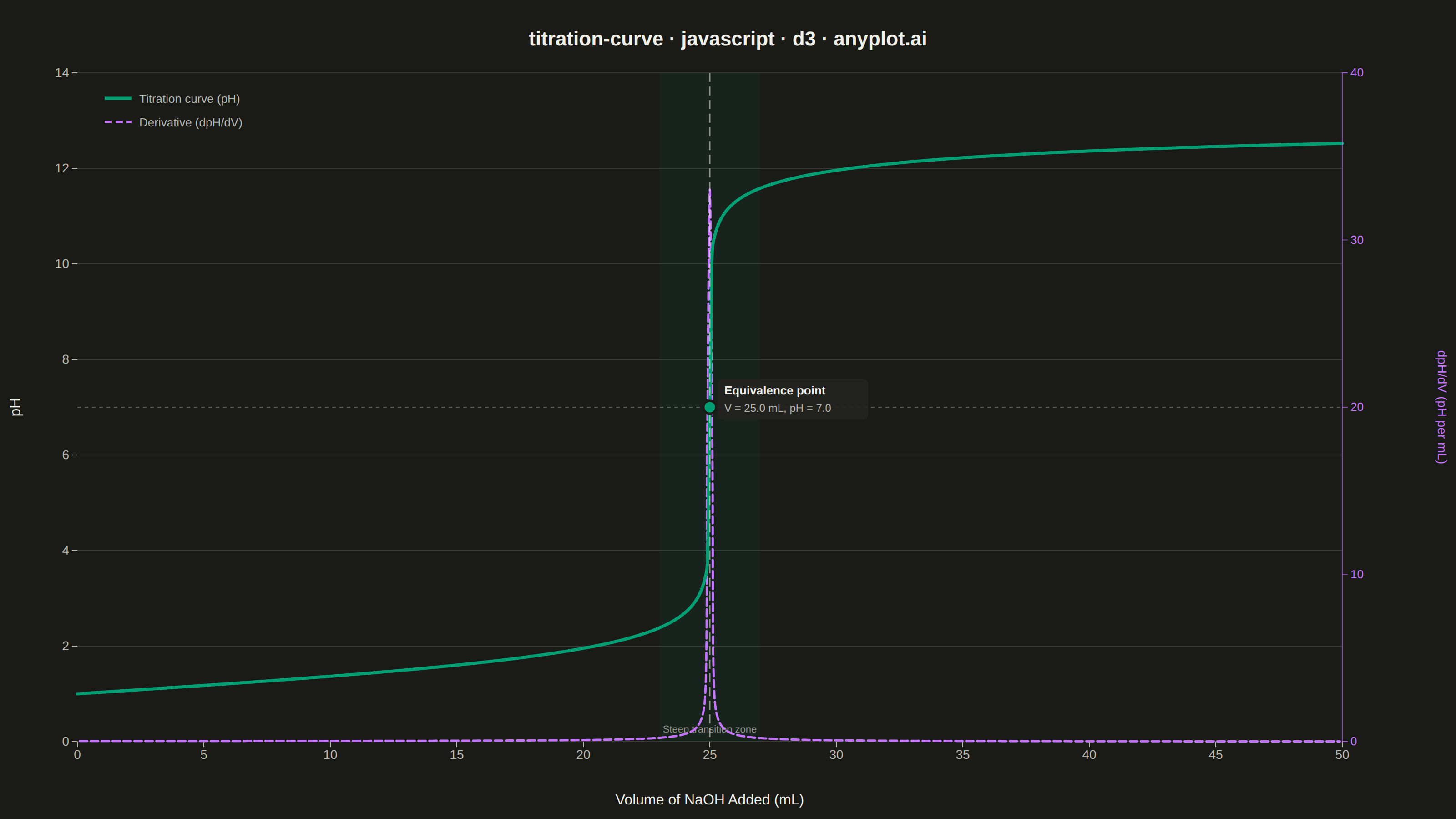
A titration curve plotting pH against volume of titrant added, producing the characteristic S-shaped (sigmoidal) curve used in analytical chemistry. The plot reveals buffer regions, equivalence points, and acid/base strength at a glance. Essential for chemistry education and laboratory analysis, it helps identify when a reaction reaches completion and which indicators are appropriate.
// anyplot.ai
// titration-curve: Acid-Base Titration Curve
// Library: d3 7.9.0 | JavaScript 22.22.3
// Quality: 90/100 | Created: 2026-06-24
//# anyplot-orientation: landscape

const t = window.ANYPLOT_TOKENS;
const { width, height } = window.ANYPLOT_SIZE;
const margin = { top: 80, right: 125, bottom: 85, left: 85 };
const iw = width - margin.left - margin.right;
const ih = height - margin.top - margin.bottom;

// --- Data: 25 mL of 0.1 M HCl titrated with 0.1 M NaOH (strong acid / strong base) ---
// 501 points: 0.0, 0.1, 0.2, … 50.0 mL
const curveData = Array.from({ length: 501 }, (_, i) => {
  const v = i * 0.1;
  const mHCl = 0.0025, mNaOH = 0.1 * v * 0.001, totalVol = (25 + v) * 0.001;
  const excess = mNaOH - mHCl;
  const ph = Math.abs(excess) < 1e-12 ? 7.0 : excess < 0 ? -Math.log10(-excess / totalVol) : 14 + Math.log10(excess / totalVol);
  return { v, ph };
});

// Central-difference numerical derivative dpH/dV (floor at 0 to suppress float noise at edges)
const derivData = curveData.slice(1, -1).map((_, i) => ({
  v: curveData[i + 1].v,
  dphdv: Math.max(0, (curveData[i + 2].ph - curveData[i].ph) / (curveData[i + 2].v - curveData[i].v)),
}));

// --- SVG ---
const svg = d3.select("#container").append("svg").attr("width", width).attr("height", height);
const g = svg.append("g").attr("transform", `translate(${margin.left},${margin.top})`);

// --- Scales ---
const xSc = d3.scaleLinear().domain([0, 50]).range([0, iw]);
const ySc = d3.scaleLinear().domain([0, 14]).range([ih, 0]);
const maxD = d3.max(derivData, (d) => d.dphdv);
const dSc = d3.scaleLinear().domain([0, Math.ceil(maxD * 1.2)]).range([ih, 0]);

// --- Gridlines (pH axis) ---
g.selectAll(".ygrid")
  .data(ySc.ticks(7))
  .join("line")
  .attr("x1", 0).attr("x2", iw)
  .attr("y1", (d) => ySc(d)).attr("y2", (d) => ySc(d))
  .attr("stroke", t.grid).attr("stroke-width", 1);

// --- pH 7 reference line ---
g.append("line")
  .attr("x1", 0).attr("x2", iw)
  .attr("y1", ySc(7)).attr("y2", ySc(7))
  .attr("stroke", t.inkSoft).attr("stroke-width", 1)
  .attr("stroke-dasharray", "4,4").attr("opacity", 0.4);

// --- Steep transition zone highlight (equivalence region) ---
const shadeX = xSc(23), shadeW = xSc(27) - xSc(23);
g.append("rect")
  .attr("x", shadeX).attr("y", 0)
  .attr("width", shadeW).attr("height", ih)
  .attr("fill", t.palette[0]).attr("opacity", 0.07);
g.append("text")
  .attr("x", shadeX + shadeW / 2).attr("y", ih - 10)
  .attr("text-anchor", "middle")
  .attr("fill", t.inkSoft).style("font-size", "11px").attr("opacity", 0.75)
  .text("Steep transition zone");

// --- Derivative curve (dpH/dV) on secondary right axis ---
g.append("path")
  .datum(derivData)
  .attr("d", d3.line().x((d) => xSc(d.v)).y((d) => dSc(d.dphdv)).curve(d3.curveCatmullRom.alpha(0.5)))
  .attr("fill", "none")
  .attr("stroke", t.palette[1])
  .attr("stroke-width", 2.5)
  .attr("stroke-dasharray", "8,4")
  .attr("stroke-linecap", "round");

// --- Titration curve (pH) ---
g.append("path")
  .datum(curveData)
  .attr("d", d3.line().x((d) => xSc(d.v)).y((d) => ySc(d.ph)).curve(d3.curveMonotoneX))
  .attr("fill", "none")
  .attr("stroke", t.palette[0])
  .attr("stroke-width", 3.5)
  .attr("stroke-linecap", "round")
  .attr("stroke-linejoin", "round");

// --- Equivalence point: vertical dashed line ---
g.append("line")
  .attr("x1", xSc(25)).attr("x2", xSc(25))
  .attr("y1", 0).attr("y2", ih)
  .attr("stroke", t.ink).attr("stroke-width", 1.5)
  .attr("stroke-dasharray", "10,5").attr("opacity", 0.55);

// --- Equivalence point marker dot ---
g.append("circle")
  .attr("cx", xSc(25)).attr("cy", ySc(7))
  .attr("r", 7).attr("fill", t.palette[0])
  .attr("stroke", t.pageBg).attr("stroke-width", 2.5);

// --- Equivalence point annotation ---
const eqX = xSc(25) + 14;
const eqY = ySc(7) - 14;
g.append("rect")
  .attr("x", eqX - 5).attr("y", eqY - 17)
  .attr("width", 165).attr("height", 44)
  .attr("fill", t.elevatedBg).attr("rx", 5).attr("opacity", 0.93);
g.append("text")
  .attr("x", eqX + 2).attr("y", eqY).attr("fill", t.ink)
  .style("font-size", "13px").style("font-weight", "600")
  .text("Equivalence point");
g.append("text")
  .attr("x", eqX + 2).attr("y", eqY + 19).attr("fill", t.inkSoft)
  .style("font-size", "12px")
  .text("V = 25.0 mL,  pH = 7.0");

// --- X axis ---
const xAx = g.append("g")
  .attr("transform", `translate(0,${ih})`)
  .call(d3.axisBottom(xSc).ticks(10).tickSize(6));
xAx.selectAll("text").attr("fill", t.inkSoft).style("font-size", "14px");
xAx.selectAll("line").attr("stroke", t.inkSoft);
xAx.select(".domain").attr("stroke", "none");

// --- Left y-axis (pH) ---
const yAxL = g.append("g").call(d3.axisLeft(ySc).ticks(7).tickSize(6));
yAxL.selectAll("text").attr("fill", t.inkSoft).style("font-size", "14px");
yAxL.selectAll("line").attr("stroke", t.inkSoft);
yAxL.select(".domain").attr("stroke", "none");

// --- Right y-axis (dpH/dV) — styled in derivative color ---
const yAxR = g.append("g")
  .attr("transform", `translate(${iw},0)`)
  .call(d3.axisRight(dSc).ticks(5).tickSize(6));
yAxR.selectAll("text").attr("fill", t.palette[1]).style("font-size", "13px");
yAxR.selectAll("line").attr("stroke", t.palette[1]).attr("opacity", 0.6);
yAxR.select(".domain").attr("stroke", t.palette[1]).attr("opacity", 0.6);

// --- Axis labels ---
svg.append("text")
  .attr("x", margin.left + iw / 2).attr("y", height - 16)
  .attr("text-anchor", "middle")
  .attr("fill", t.ink).style("font-size", "16px")
  .text("Volume of NaOH Added (mL)");

svg.append("text")
  .attr("transform", `translate(22,${margin.top + ih / 2}) rotate(-90)`)
  .attr("text-anchor", "middle")
  .attr("fill", t.ink).style("font-size", "16px")
  .text("pH");

svg.append("text")
  .attr("transform", `translate(${width - 20},${margin.top + ih / 2}) rotate(90)`)
  .attr("text-anchor", "middle")
  .attr("fill", t.palette[1]).style("font-size", "14px")
  .text("dpH/dV (pH per mL)");

// --- Legend ---
const lx = 30, ly = 20;
g.append("line")
  .attr("x1", lx).attr("x2", lx + 30).attr("y1", ly + 8).attr("y2", ly + 8)
  .attr("stroke", t.palette[0]).attr("stroke-width", 3.5);
g.append("text")
  .attr("x", lx + 38).attr("y", ly + 13).attr("fill", t.inkSoft).style("font-size", "13px")
  .text("Titration curve (pH)");

g.append("line")
  .attr("x1", lx).attr("x2", lx + 30).attr("y1", ly + 34).attr("y2", ly + 34)
  .attr("stroke", t.palette[1]).attr("stroke-width", 2.5).attr("stroke-dasharray", "8,4");
g.append("text")
  .attr("x", lx + 38).attr("y", ly + 39).attr("fill", t.inkSoft).style("font-size", "13px")
  .text("Derivative (dpH/dV)");

// --- Title ---
svg.append("text")
  .attr("x", width / 2).attr("y", 50).attr("text-anchor", "middle")
  .attr("fill", t.ink).style("font-size", "22px").style("font-weight", "600")
  .text("titration-curve · javascript · d3 · anyplot.ai");
Runnable source as JSON, for any HTTP client: https://api.anyplot.ai/specs/titration-curve/d3/code. Any spec id and library id listed in llms-full.txt fit the same URL shape; every URL below is complete and callable.
{
  "spec_id": "titration-curve",
  "language": "javascript",
  "library": "d3",
  "page": "https://anyplot.ai/titration-curve/javascript/d3",
  "hub": "https://anyplot.ai/titration-curve",
  "code_json": "https://api.anyplot.ai/specs/titration-curve/d3/code",
  "spec_json": "https://api.anyplot.ai/specs/titration-curve",
  "render_light_png": "https://storage.googleapis.com/anyplot-images/plots/titration-curve/javascript/d3/plot-light.png",
  "render_dark_png": "https://storage.googleapis.com/anyplot-images/plots/titration-curve/javascript/d3/plot-dark.png",
  "interactive_light_html": "https://storage.googleapis.com/anyplot-images/plots/titration-curve/javascript/d3/plot-light.html",
  "interactive_dark_html": "https://storage.googleapis.com/anyplot-images/plots/titration-curve/javascript/d3/plot-dark.html",
  "quality_score": 90.0,
  "license": "MIT",
  "guide": "https://anyplot.ai/llms.txt"
}
Part of Acid-Base Titration Curve on anyplot.ai.