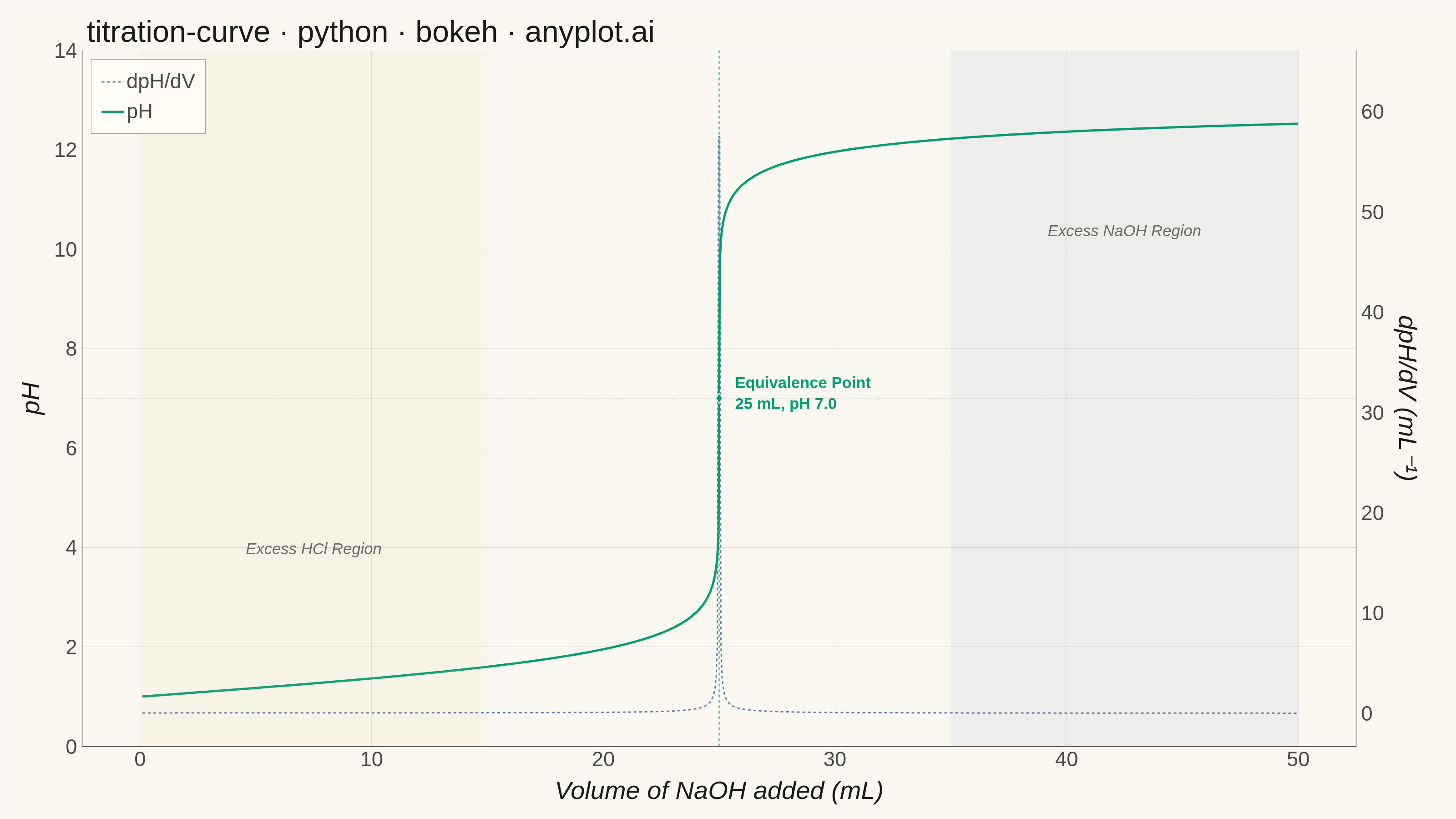
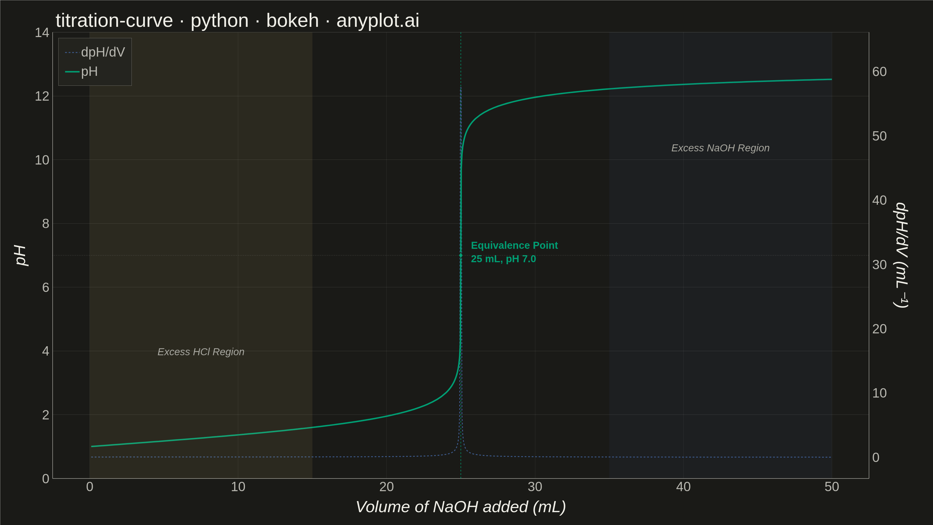
A titration curve plotting pH against volume of titrant added, producing the characteristic S-shaped (sigmoidal) curve used in analytical chemistry. The plot reveals buffer regions, equivalence points, and acid/base strength at a glance. Essential for chemistry education and laboratory analysis, it helps identify when a reaction reaches completion and which indicators are appropriate.
""" anyplot.ai
titration-curve: Acid-Base Titration Curve
Library: bokeh 3.9.1 | Python 3.13.14
Quality: 90/100 | Updated: 2026-06-24
"""

import os
import sys
import time
from pathlib import Path


# Prevent this file from shadowing the installed bokeh package
_here = os.path.dirname(os.path.abspath(__file__))
sys.path = [p for p in sys.path if os.path.abspath(p) != _here]

import numpy as np
from bokeh.io import output_file, save
from bokeh.models import BoxAnnotation, ColumnDataSource, HoverTool, Label, LinearAxis, Range1d, Span
from bokeh.plotting import figure
from selenium import webdriver
from selenium.webdriver.chrome.options import Options


THEME = os.getenv("ANYPLOT_THEME", "light")

# Theme-adaptive chrome tokens
PAGE_BG = "#FAF8F1" if THEME == "light" else "#1A1A17"
ELEVATED_BG = "#FFFDF6" if THEME == "light" else "#242420"
INK = "#1A1A17" if THEME == "light" else "#F0EFE8"
INK_SOFT = "#4A4A44" if THEME == "light" else "#B8B7B0"
INK_MUTED = "#6B6A63" if THEME == "light" else "#A8A79F"

# Imprint palette — canonical order, first series always #009E73
IMPRINT_PALETTE = ["#009E73", "#C475FD", "#4467A3", "#BD8233", "#AE3030", "#2ABCCD", "#954477", "#99B314"]
ANYPLOT_AMBER = "#DDCC77"  # warning / caution anchor

CURVE_COLOR = IMPRINT_PALETTE[0]  # #009E73 — pH titration curve (first series)
DERIV_COLOR = IMPRINT_PALETTE[2]  # #4467A3 — dpH/dV derivative (third series, blue)
EQ_COLOR = IMPRINT_PALETTE[0]  # #009E73 — equivalence point (tied to main curve)
ACID_FILL = ANYPLOT_AMBER  # amber — excess acid region (caution/warm semantic)
BASE_FILL = IMPRINT_PALETTE[2]  # #4467A3 — excess base region (cool/alkaline semantic)

# ── Data: 25 mL of 0.1 M HCl titrated with 0.1 M NaOH ──────────────────────
acid_volume_ml = 25.0
acid_conc = 0.1
base_conc = 0.1
eq_vol = acid_volume_ml * acid_conc / base_conc  # 25 mL equivalence

volume_ml = np.unique(
    np.concatenate(
        [
            np.linspace(0.1, 24.0, 80),
            np.linspace(24.0, 26.0, 40),  # dense around equivalence point
            np.linspace(26.0, 50.0, 80),
        ]
    )
)

moles_acid = acid_conc * acid_volume_ml / 1000
moles_base = base_conc * volume_ml / 1000
total_vol_L = (acid_volume_ml + volume_ml) / 1000

ph = np.empty_like(volume_ml)
for i in range(len(volume_ml)):
    if moles_base[i] < moles_acid - 1e-10:
        h_plus = (moles_acid - moles_base[i]) / total_vol_L[i]
        ph[i] = -np.log10(h_plus)
    elif moles_base[i] > moles_acid + 1e-10:
        oh_minus = (moles_base[i] - moles_acid) / total_vol_L[i]
        ph[i] = 14.0 + np.log10(oh_minus)
    else:
        ph[i] = 7.0

# Derivative dpH/dV — central differences
dph_dv = np.gradient(ph, volume_ml)
dph_dv = np.where(np.isfinite(dph_dv), dph_dv, 0.0)
eq_ph = 7.0

source = ColumnDataSource(data={"volume": volume_ml, "ph": ph, "dph_dv": dph_dv})

# ── Canvas: landscape 3200×1800 (hard rule, no deviation) ───────────────────
W, H = 3200, 1800

p = figure(
    width=W,
    height=H,
    x_axis_label="Volume of NaOH added (mL)",
    y_axis_label="pH",
    y_range=Range1d(0, 14),
    title="titration-curve · python · bokeh · anyplot.ai",
    toolbar_location=None,  # keep PNG dimensions exact; HTML retains interactivity via output_file
    min_border_bottom=160,  # 34pt tick labels + 42pt axis label
    min_border_left=180,  # 34pt tick labels + 42pt axis label
    min_border_top=110,  # 50pt title
    min_border_right=220,  # right-side dpH/dV axis (label + ticks)
)

# ── Buffer region shading ────────────────────────────────────────────────────
p.add_layout(BoxAnnotation(left=0, right=15, fill_color=ACID_FILL, fill_alpha=0.09, line_color=None))
p.add_layout(BoxAnnotation(left=35, right=50, fill_color=BASE_FILL, fill_alpha=0.07, line_color=None))

# Region labels (theme-adaptive muted ink)
p.add_layout(
    Label(
        x=7.5,
        y=3.8,
        text="Excess HCl Region",
        text_font_size="26pt",
        text_color=INK_MUTED,
        text_align="center",
        text_font_style="italic",
    )
)
p.add_layout(
    Label(
        x=42.5,
        y=10.2,
        text="Excess NaOH Region",
        text_font_size="26pt",
        text_color=INK_MUTED,
        text_align="center",
        text_font_style="italic",
    )
)

# ── Secondary y-axis for derivative (right side) ────────────────────────────
deriv_max = float(np.max(dph_dv)) * 1.15
p.extra_y_ranges = {"deriv": Range1d(start=-deriv_max * 0.05, end=deriv_max)}
deriv_axis = LinearAxis(
    y_range_name="deriv",
    axis_label="dpH/dV (mL⁻¹)",
    axis_label_text_font_size="42pt",
    axis_label_text_color=DERIV_COLOR,
    major_label_text_font_size="34pt",
    major_label_text_color=DERIV_COLOR,
    axis_line_color=DERIV_COLOR,
    major_tick_line_color=None,
    minor_tick_line_color=None,
)
p.add_layout(deriv_axis, "right")

# ── Derivative curve (dashed, secondary axis) ────────────────────────────────
p.line(
    "volume",
    "dph_dv",
    source=ColumnDataSource(data={"volume": volume_ml, "dph_dv": dph_dv}),
    line_width=3,
    color=DERIV_COLOR,
    line_alpha=0.85,
    line_dash="dashed",
    y_range_name="deriv",
    legend_label="dpH/dV",
)

# ── Main titration curve (solid, prominent) ──────────────────────────────────
p.line("volume", "ph", source=source, line_width=5, color=CURVE_COLOR, legend_label="pH")

# ── Equivalence point ─────────────────────────────────────────────────────────
p.add_layout(
    Span(location=eq_vol, dimension="height", line_color=EQ_COLOR, line_width=2.5, line_dash="dashed", line_alpha=0.7)
)
p.scatter([eq_vol], [eq_ph], size=22, color=EQ_COLOR, marker="diamond", line_color=PAGE_BG, line_width=2)
p.add_layout(
    Label(
        x=eq_vol,
        y=eq_ph,
        text=f"Equivalence Point\n{eq_vol:.0f} mL, pH {eq_ph:.1f}",
        text_font_size="26pt",
        text_font_style="bold",
        text_color=EQ_COLOR,
        x_offset=35,
        y_offset=-30,
    )
)

# ── pH 7 neutral reference line ──────────────────────────────────────────────
p.add_layout(
    Span(location=7, dimension="width", line_color=INK_MUTED, line_width=1.5, line_dash="dotted", line_alpha=0.4)
)

# ── Hover tooltip ─────────────────────────────────────────────────────────────
p.add_tools(
    HoverTool(tooltips=[("Volume", "@volume{0.1} mL"), ("pH", "@ph{0.2}")], mode="vline", line_policy="nearest")
)

# ── Font sizes (bokeh native-pixel: 50pt title, 42pt axis, 34pt ticks) ──────
p.title.text_font_size = "50pt"
p.title.text_font_style = "normal"
p.title.text_color = INK
p.title.offset = 10

p.xaxis.axis_label_text_font_size = "42pt"
p.yaxis.axis_label_text_font_size = "42pt"
p.xaxis.major_label_text_font_size = "34pt"
p.yaxis.major_label_text_font_size = "34pt"
p.xaxis.axis_label_standoff = 18
p.yaxis.axis_label_standoff = 18

# ── Theme-adaptive chrome ─────────────────────────────────────────────────────
p.xaxis.axis_label_text_color = INK
p.yaxis.axis_label_text_color = INK
p.xaxis.major_label_text_color = INK_SOFT
p.yaxis.major_label_text_color = INK_SOFT
p.xaxis.axis_line_color = INK_SOFT
p.yaxis.axis_line_color = INK_SOFT
p.xaxis.axis_line_width = 1.5
p.yaxis.axis_line_width = 1.5
p.xaxis.major_tick_line_color = None
p.yaxis.major_tick_line_color = None
p.xaxis.minor_tick_line_color = None
p.yaxis.minor_tick_line_color = None

p.outline_line_color = None
p.background_fill_color = PAGE_BG
p.border_fill_color = PAGE_BG

p.ygrid.grid_line_color = INK
p.ygrid.grid_line_alpha = 0.15
p.ygrid.grid_line_width = 1
p.xgrid.grid_line_color = INK
p.xgrid.grid_line_alpha = 0.10
p.xgrid.grid_line_width = 1

# ── Legend ────────────────────────────────────────────────────────────────────
p.legend.location = "top_left"
p.legend.label_text_font_size = "34pt"
p.legend.label_text_color = INK_SOFT
p.legend.glyph_height = 35
p.legend.glyph_width = 50
p.legend.spacing = 14
p.legend.padding = 22
p.legend.margin = 20
p.legend.background_fill_alpha = 0.92
p.legend.background_fill_color = ELEVATED_BG
p.legend.border_line_color = INK_SOFT
p.legend.border_line_width = 1.5

# ── Save HTML (interactive artifact) then screenshot via Selenium ────────────
output_file(f"plot-{THEME}.html")
save(p)

opts = Options()
for arg in (
    "--headless=new",
    "--no-sandbox",
    "--disable-dev-shm-usage",
    "--disable-gpu",
    f"--window-size={W},{H}",
    "--hide-scrollbars",
):
    opts.add_argument(arg)

driver = webdriver.Chrome(options=opts)
# Force the viewport to the exact canvas size via CDP (headless=new outer vs inner window differs)
driver.execute_cdp_cmd(
    "Emulation.setDeviceMetricsOverride", {"width": W, "height": H, "deviceScaleFactor": 1, "mobile": False}
)
driver.get(f"file://{Path(f'plot-{THEME}.html').resolve()}")
time.sleep(3)  # let bokeh JS render the canvas
driver.save_screenshot(f"plot-{THEME}.png")
driver.quit()
Runnable source as JSON, for any HTTP client: https://api.anyplot.ai/specs/titration-curve/bokeh/code. Any spec id and library id listed in llms-full.txt fit the same URL shape; every URL below is complete and callable.
{
  "spec_id": "titration-curve",
  "language": "python",
  "library": "bokeh",
  "page": "https://anyplot.ai/titration-curve/python/bokeh",
  "hub": "https://anyplot.ai/titration-curve",
  "code_json": "https://api.anyplot.ai/specs/titration-curve/bokeh/code",
  "spec_json": "https://api.anyplot.ai/specs/titration-curve",
  "render_light_png": "https://storage.googleapis.com/anyplot-images/plots/titration-curve/python/bokeh/plot-light.png",
  "render_dark_png": "https://storage.googleapis.com/anyplot-images/plots/titration-curve/python/bokeh/plot-dark.png",
  "interactive_light_html": "https://storage.googleapis.com/anyplot-images/plots/titration-curve/python/bokeh/plot-light.html",
  "interactive_dark_html": "https://storage.googleapis.com/anyplot-images/plots/titration-curve/python/bokeh/plot-dark.html",
  "quality_score": 90.0,
  "license": "MIT",
  "guide": "https://anyplot.ai/llms.txt"
}
Part of Acid-Base Titration Curve on anyplot.ai.