The same plot in 14 other libraries — Python: Altair, Bokeh, lets-plot, Matplotlib, Plotly, plotnine, Pygal, Seaborn; Julia: Makie.jl; JavaScript: Chart.js, D3.js, Apache ECharts, Highcharts, MUI X Charts. Compare all 15 side by side: Acid-Base Titration Curve in Python, R, Julia and JavaScript.
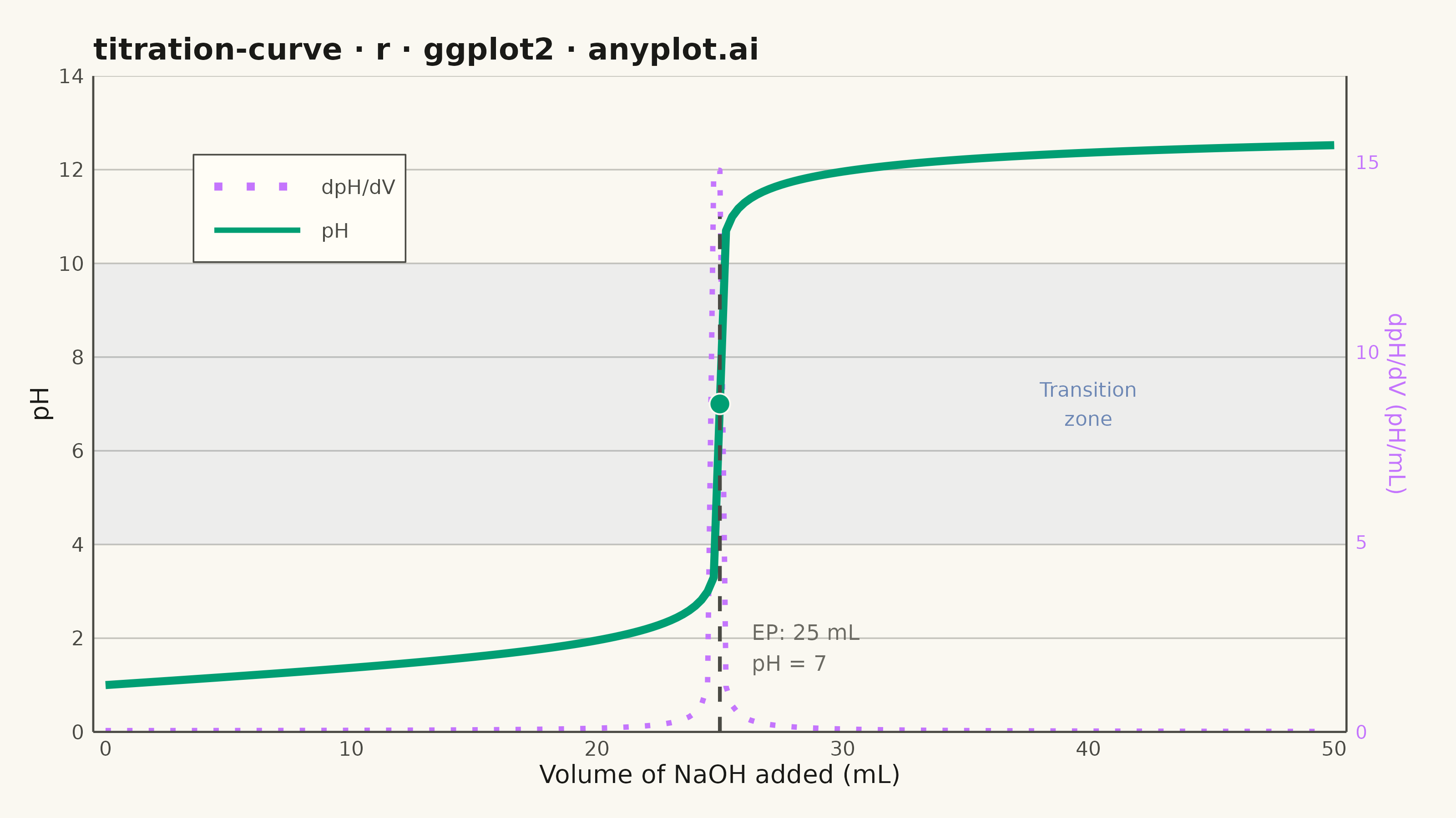
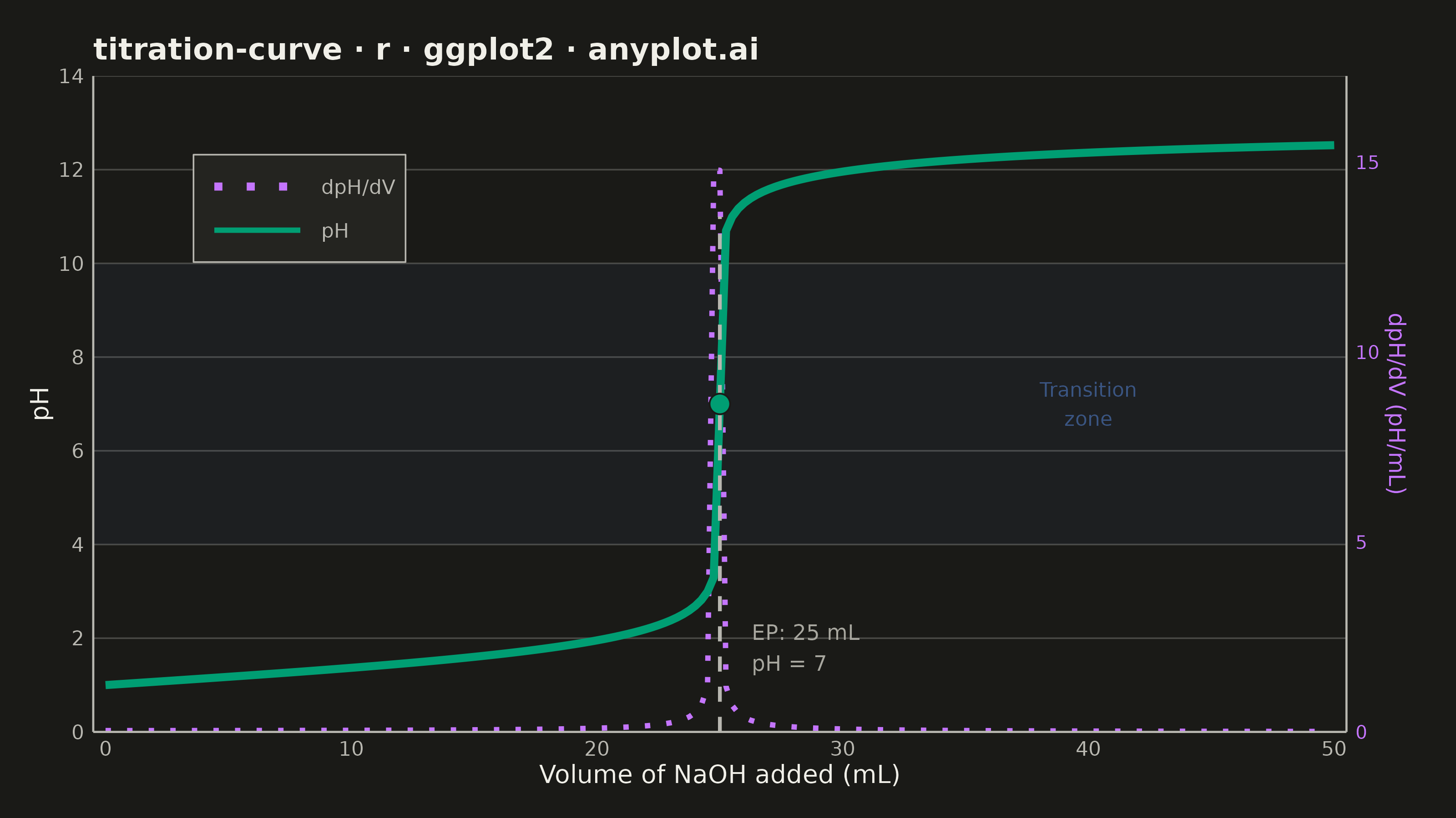
A titration curve plotting pH against volume of titrant added, producing the characteristic S-shaped (sigmoidal) curve used in analytical chemistry. The plot reveals buffer regions, equivalence points, and acid/base strength at a glance. Essential for chemistry education and laboratory analysis, it helps identify when a reaction reaches completion and which indicators are appropriate.
#' anyplot.ai
#' titration-curve: Acid-Base Titration Curve
#' Library: ggplot2 3.5.1 | R 4.4.1
#' Quality: 90/100 | Created: 2026-06-24

library(ggplot2)
library(ragg)

# Theme tokens (Imprint palette, theme-adaptive chrome)
THEME       <- Sys.getenv("ANYPLOT_THEME", "light")
PAGE_BG     <- if (THEME == "light") "#FAF8F1" else "#1A1A17"
ELEVATED_BG <- if (THEME == "light") "#FFFDF6" else "#242420"
INK         <- if (THEME == "light") "#1A1A17" else "#F0EFE8"
INK_SOFT    <- if (THEME == "light") "#4A4A44" else "#B8B7B0"
INK_MUTED   <- if (THEME == "light") "#6B6A63" else "#A8A79F"
GRID_COLOR  <- if (THEME == "light") "#C5C4BD" else "#494945"
IMPRINT_PALETTE <- c(
  "#009E73",  # 1 brand green — titration curve (first series, always)
  "#C475FD",  # 2 lavender    — derivative overlay
  "#4467A3",  # 3 blue
  "#BD8233",  # 4 ochre
  "#AE3030",  # 5 matte red
  "#2ABCCD",  # 6 cyan
  "#954477",  # 7 rose
  "#99B314"   # 8 lime
)

# Data: 25 mL of 0.1 M HCl titrated with 0.1 M NaOH
c_acid   <- 0.1    # mol/L
v_acid   <- 25.0   # mL
c_base   <- 0.1    # mol/L
vol_step <- 0.25   # mL

volume_ml <- seq(0, 50, by = vol_step)
mmol_acid <- c_acid * v_acid  # 2.5 mmol

mmol_base <- c_base * volume_ml
total_vol <- v_acid + volume_ml
excess    <- mmol_acid - mmol_base

pH <- ifelse(
  abs(excess) < 1e-9,
  7.0,
  ifelse(excess > 0, -log10(abs(excess) / total_vol), 14 + log10(abs(excess) / total_vol))
)

# Derivative dpH/dV (forward finite difference; last point set to NA)
dphdv_raw <- c(diff(pH) / diff(volume_ml), NA_real_)

# Scale derivative to primary axis range [0, 12] — leaves headroom below pH 14
max_dphdv    <- max(dphdv_raw, na.rm = TRUE)
dphdv_scaled <- dphdv_raw / max_dphdv * 12

df <- data.frame(
  volume_ml    = volume_ml,
  pH           = pH,
  dphdv_scaled = dphdv_scaled
)

# Equivalence point: 25 mL NaOH, pH 7 for strong acid/base
equiv_vol <- v_acid
equiv_ph  <- 7.0

# Secondary axis breaks in dpH/dV units
sec_breaks <- pretty(c(0, max_dphdv), n = 5)

# Title — 42 chars (< 67 baseline), no font-size scaling required
title_str <- "titration-curve · r · ggplot2 · anyplot.ai"

p <- ggplot(df, aes(x = volume_ml)) +
  # Steep-slope transition zone (pH 4–10): key region around equivalence
  annotate("rect",
    xmin = -Inf, xmax = Inf,
    ymin = 4, ymax = 10,
    fill = IMPRINT_PALETTE[3], alpha = 0.07
  ) +
  # Derivative overlay (scaled to primary axis, dotted)
  geom_line(
    aes(y = dphdv_scaled, color = "dpH/dV", linetype = "dpH/dV"),
    linewidth = 1.0, na.rm = TRUE
  ) +
  # Main titration curve
  geom_line(
    aes(y = pH, color = "pH", linetype = "pH"),
    linewidth = 1.5
  ) +
  # Equivalence point: vertical dashed line (capped at y=11 so derivative spike has breathing room)
  annotate("segment",
    x = equiv_vol, xend = equiv_vol,
    y = 0,         yend = 11,
    linetype  = "dashed",
    color     = INK_SOFT,
    linewidth = 0.7
  ) +
  # Equivalence point dot on the curve
  annotate("point",
    x     = equiv_vol,
    y     = equiv_ph,
    shape = 21,
    size  = 3.5,
    fill  = IMPRINT_PALETTE[1],
    color = PAGE_BG
  ) +
  # Equivalence point text annotation
  annotate("text",
    x     = equiv_vol + 1.3,
    y     = 1.8,
    label = paste0("EP: ", equiv_vol, " mL\npH = ", equiv_ph),
    hjust = 0,
    size  = 3.0,
    color = INK_MUTED
  ) +
  # Transition zone label (right side, in empty area above plateau)
  annotate("text",
    x     = 40,
    y     = 7.0,
    label = "Transition\nzone",
    hjust = 0.5,
    size  = 2.8,
    color = IMPRINT_PALETTE[3],
    alpha = 0.75
  ) +
  # Color + linetype scales (merged into single legend)
  scale_color_manual(
    name   = NULL,
    values = c("pH" = IMPRINT_PALETTE[1], "dpH/dV" = IMPRINT_PALETTE[2]),
    guide  = guide_legend(override.aes = list(linewidth = c(1.5, 1.0)))
  ) +
  scale_linetype_manual(
    name   = NULL,
    values = c("pH" = "solid", "dpH/dV" = "dotted")
  ) +
  # Dual y-axis: pH primary, dpH/dV secondary
  scale_y_continuous(
    name     = "pH",
    limits   = c(0, 14),
    breaks   = seq(0, 14, by = 2),
    expand   = expansion(0, 0),
    sec.axis = sec_axis(
      ~ . * max_dphdv / 12,
      name   = "dpH/dV (pH/mL)",
      breaks = sec_breaks
    )
  ) +
  scale_x_continuous(
    name   = "Volume of NaOH added (mL)",
    limits = c(0, 50),
    breaks = seq(0, 50, by = 10),
    expand = expansion(0.01, 0)
  ) +
  labs(title = title_str) +
  theme_minimal(base_size = 8) +
  theme(
    plot.background     = element_rect(fill = PAGE_BG,  color = PAGE_BG),
    panel.background    = element_rect(fill = PAGE_BG,  color = NA),
    panel.grid.major.x  = element_blank(),
    panel.grid.major.y  = element_line(color = GRID_COLOR, linewidth = 0.3),
    panel.grid.minor    = element_blank(),
    panel.border        = element_blank(),
    axis.title.x        = element_text(color = INK,                size = 10),
    axis.title.y.left   = element_text(color = INK,                size = 10),
    axis.title.y.right  = element_text(color = IMPRINT_PALETTE[2], size = 9),
    axis.text.x         = element_text(color = INK_SOFT,           size = 8),
    axis.text.y.left    = element_text(color = INK_SOFT,           size = 8),
    axis.text.y.right   = element_text(color = IMPRINT_PALETTE[2], size = 7.5),
    axis.line.x         = element_line(color = INK_SOFT, linewidth = 0.4),
    axis.line.y         = element_line(color = INK_SOFT, linewidth = 0.4),
    plot.title          = element_text(color = INK, size = 12, face = "bold"),
    legend.background   = element_rect(fill = ELEVATED_BG, color = INK_SOFT, linewidth = 0.3),
    legend.text         = element_text(color = INK_SOFT, size = 8),
    legend.key.width    = unit(1.5, "cm"),
    legend.position        = "inside",
    legend.position.inside = c(0.08, 0.88),
    legend.justification   = c(0, 1),
    plot.margin         = margin(15, 20, 12, 12)
  )

ggsave(
  filename = sprintf("plot-%s.png", THEME),
  plot     = p,
  device   = ragg::agg_png,
  width    = 8,
  height   = 4.5,
  units    = "in",
  dpi      = 400
)
Runnable source as JSON, for any HTTP client: https://api.anyplot.ai/specs/titration-curve/ggplot2/code. Any spec id and library id listed in llms-full.txt fit the same URL shape; every URL below is complete and callable.
{
  "spec_id": "titration-curve",
  "language": "r",
  "library": "ggplot2",
  "page": "https://anyplot.ai/titration-curve/r/ggplot2",
  "hub": "https://anyplot.ai/titration-curve",
  "code_json": "https://api.anyplot.ai/specs/titration-curve/ggplot2/code",
  "spec_json": "https://api.anyplot.ai/specs/titration-curve",
  "render_light_png": "https://storage.googleapis.com/anyplot-images/plots/titration-curve/r/ggplot2/plot-light.png",
  "render_dark_png": "https://storage.googleapis.com/anyplot-images/plots/titration-curve/r/ggplot2/plot-dark.png",
  "quality_score": 90.0,
  "license": "MIT",
  "guide": "https://anyplot.ai/llms.txt"
}
Part of Acid-Base Titration Curve on anyplot.ai.