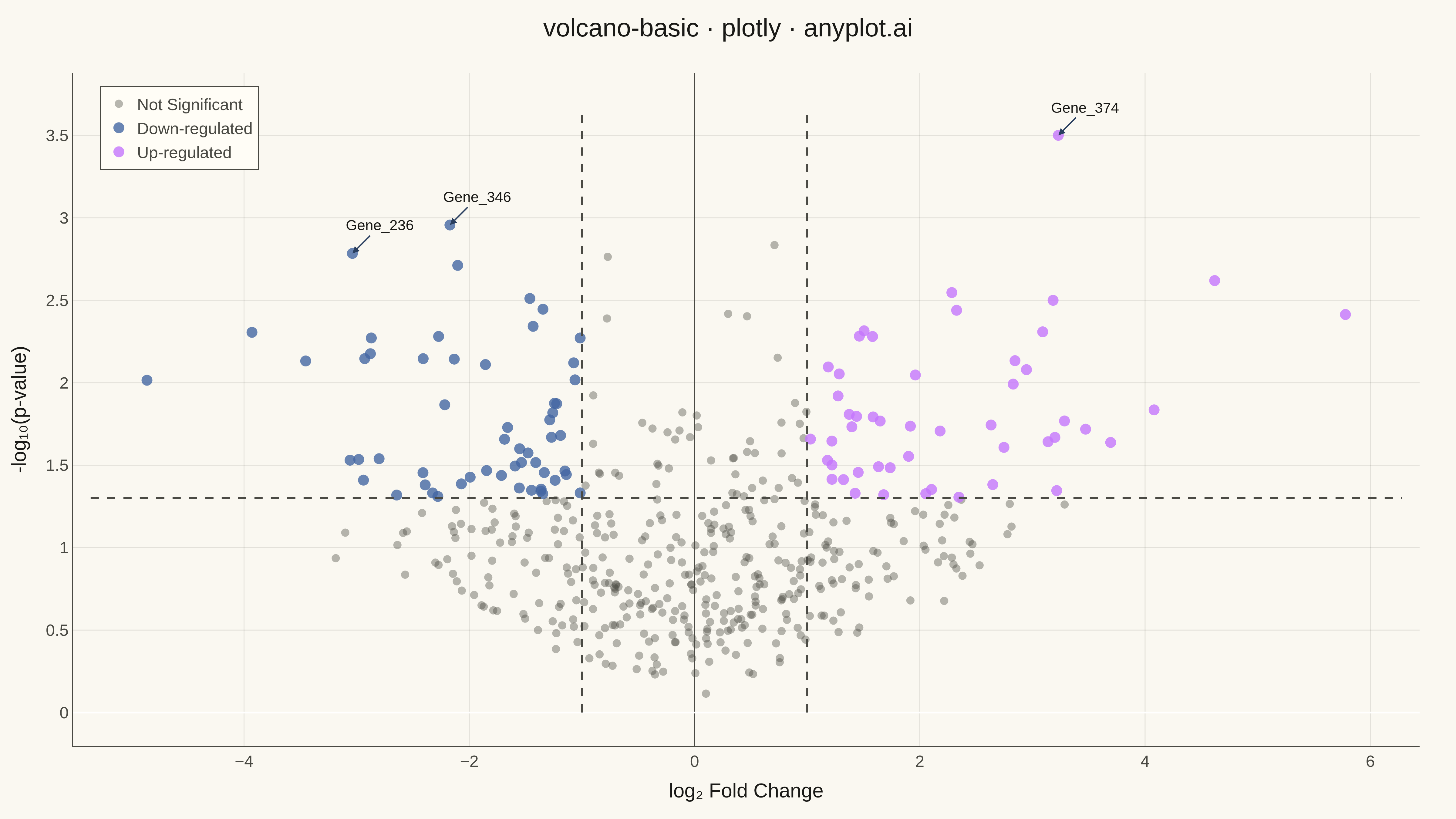
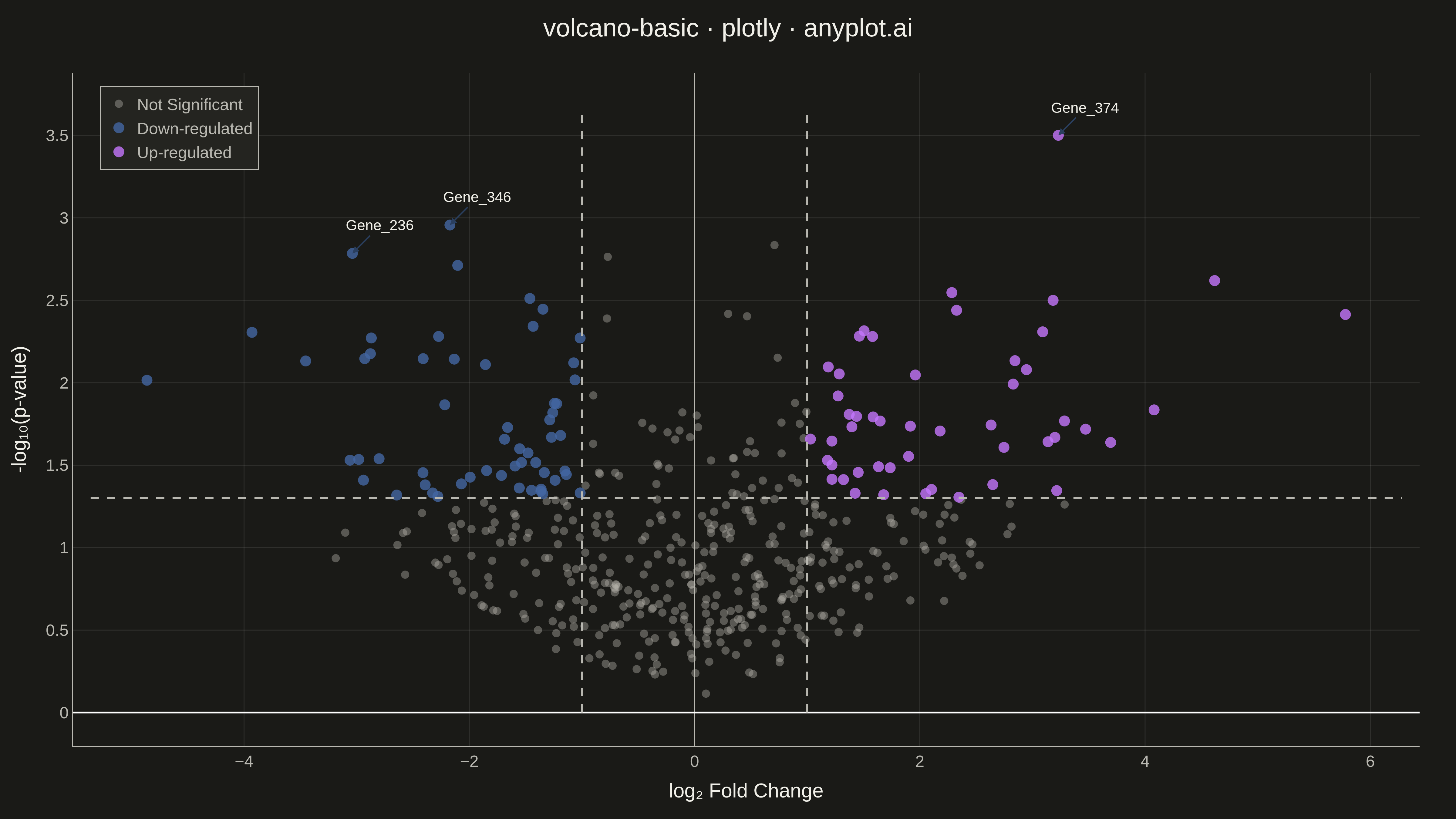
A volcano plot displays statistical significance (-log10 p-value) on the y-axis versus effect size (log2 fold change) on the x-axis. Points are typically color-coded to highlight features that are both statistically significant and have large effect sizes. This visualization is essential for quickly identifying the most important changes in differential expression, proteomics, and genomics studies.
""" anyplot.ai
volcano-basic: Volcano Plot for Statistical Significance
Library: plotly 6.7.0 | Python 3.13.13
Quality: 93/100 | Updated: 2026-05-14
"""

import os

import numpy as np
import plotly.graph_objects as go


# Theme tokens
THEME = os.getenv("ANYPLOT_THEME", "light")
PAGE_BG = "#FAF8F1" if THEME == "light" else "#1A1A17"
ELEVATED_BG = "#FFFDF6" if THEME == "light" else "#242420"
INK = "#1A1A17" if THEME == "light" else "#F0EFE8"
INK_SOFT = "#4A4A44" if THEME == "light" else "#B8B7B0"
GRID = "rgba(26,26,23,0.10)" if THEME == "light" else "rgba(240,239,232,0.10)"

# Okabe-Ito palette
OKABE_ITO_VERMILLION = "#C475FD"  # Position 2 - red/orange for up-regulated
OKABE_ITO_BLUE = "#4467A3"  # Position 3 - blue for down-regulated

# Data - Simulated differential gene expression results
np.random.seed(42)
n_genes = 500

# Generate log2 fold changes
log2_fold_change = np.random.normal(0, 1.5, n_genes)

# Generate p-values (most non-significant, some significant)
base_pvalues = np.random.beta(1, 3, n_genes)
effect_boost = np.abs(log2_fold_change) / 5
pvalues = base_pvalues * np.exp(-effect_boost * 3)
pvalues = np.clip(pvalues, 1e-20, 1)

# Transform to -log10 scale
neg_log10_pvalue = -np.log10(pvalues)

# Define significance thresholds
fc_threshold = 1.0  # log2 fold change threshold
pval_threshold = 0.05
neg_log10_threshold = -np.log10(pval_threshold)

# Classify points
sig_up = (log2_fold_change > fc_threshold) & (neg_log10_pvalue > neg_log10_threshold)
sig_down = (log2_fold_change < -fc_threshold) & (neg_log10_pvalue > neg_log10_threshold)
non_sig = ~(sig_up | sig_down)

# Gene names
gene_names = [f"Gene_{i}" for i in range(n_genes)]

# Create figure
fig = go.Figure()

# Non-significant points (adaptive neutral gray)
fig.add_trace(
    go.Scatter(
        x=log2_fold_change[non_sig],
        y=neg_log10_pvalue[non_sig],
        mode="markers",
        marker=dict(size=9, color=INK_SOFT, opacity=0.4),
        name="Not Significant",
        hovertemplate="%{text}<br>log₂FC: %{x:.2f}<br>-log₁₀(p): %{y:.2f}<extra></extra>",
        text=[gene_names[i] for i in np.where(non_sig)[0]],
    )
)

# Significant down-regulated (Okabe-Ito blue)
fig.add_trace(
    go.Scatter(
        x=log2_fold_change[sig_down],
        y=neg_log10_pvalue[sig_down],
        mode="markers",
        marker=dict(size=12, color=OKABE_ITO_BLUE, opacity=0.8),
        name="Down-regulated",
        hovertemplate="%{text}<br>log₂FC: %{x:.2f}<br>-log₁₀(p): %{y:.2f}<extra></extra>",
        text=[gene_names[i] for i in np.where(sig_down)[0]],
    )
)

# Significant up-regulated (Okabe-Ito vermillion)
fig.add_trace(
    go.Scatter(
        x=log2_fold_change[sig_up],
        y=neg_log10_pvalue[sig_up],
        mode="markers",
        marker=dict(size=12, color=OKABE_ITO_VERMILLION, opacity=0.8),
        name="Up-regulated",
        hovertemplate="%{text}<br>log₂FC: %{x:.2f}<br>-log₁₀(p): %{y:.2f}<extra></extra>",
        text=[gene_names[i] for i in np.where(sig_up)[0]],
    )
)

# Horizontal threshold line (p-value = 0.05)
x_range = [min(log2_fold_change) - 0.5, max(log2_fold_change) + 0.5]
fig.add_trace(
    go.Scatter(
        x=x_range,
        y=[neg_log10_threshold, neg_log10_threshold],
        mode="lines",
        line=dict(color=INK_SOFT, width=2, dash="dash"),
        showlegend=False,
    )
)

# Vertical threshold lines (fold change = ±1)
y_range = [0, max(neg_log10_pvalue) * 1.05]
fig.add_trace(
    go.Scatter(
        x=[-fc_threshold, -fc_threshold],
        y=y_range,
        mode="lines",
        line=dict(color=INK_SOFT, width=2, dash="dash"),
        showlegend=False,
    )
)
fig.add_trace(
    go.Scatter(
        x=[fc_threshold, fc_threshold],
        y=y_range,
        mode="lines",
        line=dict(color=INK_SOFT, width=2, dash="dash"),
        showlegend=False,
    )
)

# Label top significant genes
top_indices = np.argsort(neg_log10_pvalue)[-5:]
annotations = []
for idx in top_indices:
    if sig_up[idx] or sig_down[idx]:
        annotations.append(
            dict(
                x=log2_fold_change[idx],
                y=neg_log10_pvalue[idx],
                text=gene_names[idx],
                showarrow=True,
                arrowhead=2,
                arrowsize=1,
                arrowwidth=1.5,
                ax=30,
                ay=-30,
                font=dict(size=16, color=INK),
            )
        )

# Update layout
fig.update_layout(
    title=dict(text="volcano-basic · plotly · anyplot.ai", font=dict(size=28, color=INK), x=0.5, xanchor="center"),
    xaxis=dict(
        title=dict(text="log₂ Fold Change", font=dict(size=22, color=INK)),
        tickfont=dict(size=18, color=INK_SOFT),
        zeroline=True,
        zerolinewidth=1,
        zerolinecolor=INK_SOFT,
        gridcolor=GRID,
        linecolor=INK_SOFT,
    ),
    yaxis=dict(
        title=dict(text="-log₁₀(p-value)", font=dict(size=22, color=INK)),
        tickfont=dict(size=18, color=INK_SOFT),
        gridcolor=GRID,
        linecolor=INK_SOFT,
    ),
    paper_bgcolor=PAGE_BG,
    plot_bgcolor=PAGE_BG,
    font=dict(color=INK),
    legend=dict(
        font=dict(size=18, color=INK_SOFT), x=0.02, y=0.98, bgcolor=ELEVATED_BG, bordercolor=INK_SOFT, borderwidth=1
    ),
    annotations=annotations,
    margin=dict(l=80, r=40, t=80, b=80),
)

# Save as PNG (4800 x 2700 px)
fig.write_image(f"plot-{THEME}.png", width=1600, height=900, scale=3)

# Save interactive HTML version
fig.write_html(f"plot-{THEME}.html", include_plotlyjs="cdn")
Runnable source as JSON, for any HTTP client: https://api.anyplot.ai/specs/volcano-basic/plotly/code. Any spec id and library id listed in llms-full.txt fit the same URL shape; every URL below is complete and callable.
{
  "spec_id": "volcano-basic",
  "language": "python",
  "library": "plotly",
  "page": "https://anyplot.ai/volcano-basic/python/plotly",
  "hub": "https://anyplot.ai/volcano-basic",
  "code_json": "https://api.anyplot.ai/specs/volcano-basic/plotly/code",
  "spec_json": "https://api.anyplot.ai/specs/volcano-basic",
  "render_light_png": "https://storage.googleapis.com/anyplot-images/plots/volcano-basic/python/plotly/plot-light.png",
  "render_dark_png": "https://storage.googleapis.com/anyplot-images/plots/volcano-basic/python/plotly/plot-dark.png",
  "interactive_light_html": "https://storage.googleapis.com/anyplot-images/plots/volcano-basic/python/plotly/plot-light.html",
  "interactive_dark_html": "https://storage.googleapis.com/anyplot-images/plots/volcano-basic/python/plotly/plot-dark.html",
  "quality_score": 93.0,
  "license": "MIT",
  "guide": "https://anyplot.ai/llms.txt"
}
Part of Volcano Plot for Statistical Significance on anyplot.ai.