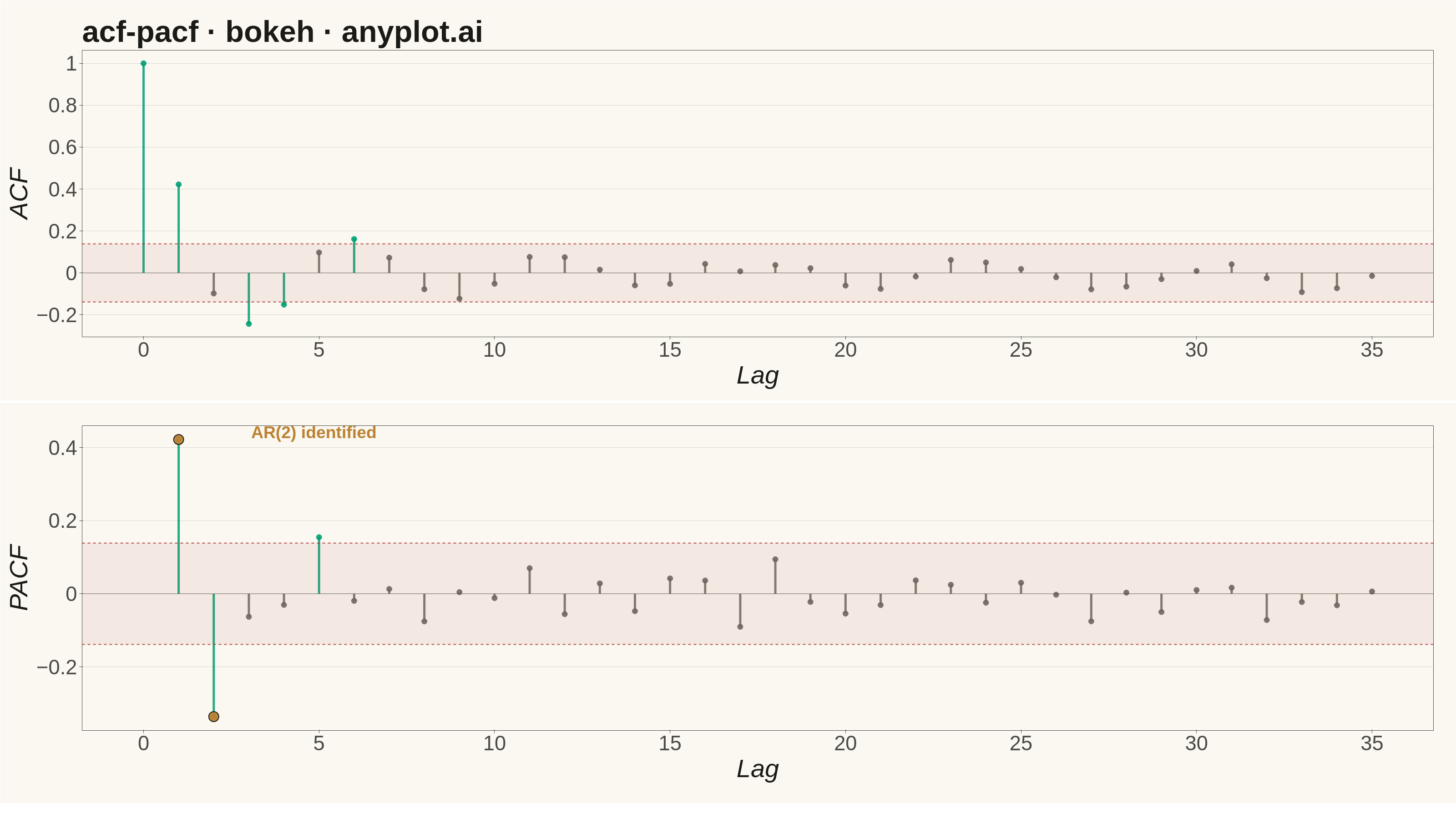
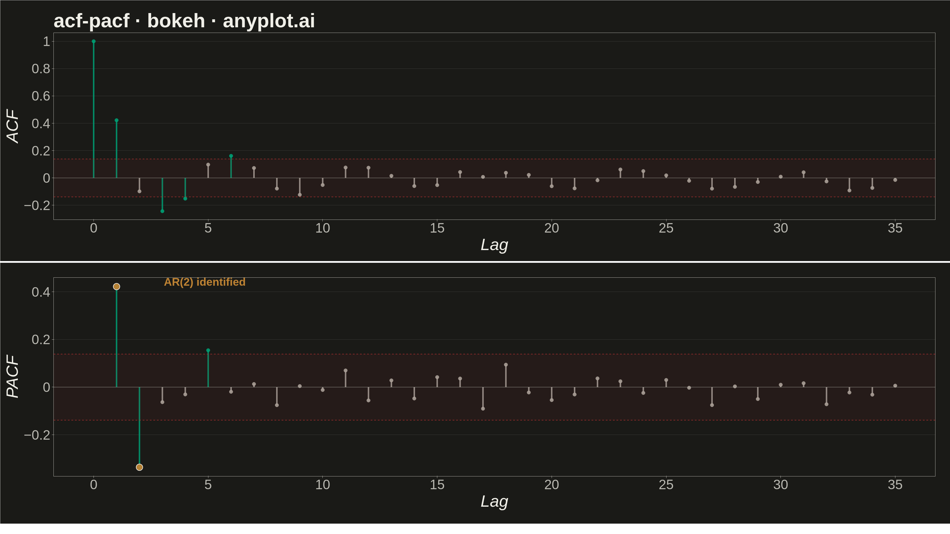
Displays the autocorrelation function (ACF) and partial autocorrelation function (PACF) of a time series as vertical stem/bar plots arranged in two vertically stacked subplots. Each lag is represented by a vertical line from zero to the correlation value, with horizontal dashed lines indicating 95% confidence bounds. These plots are essential for identifying the order of AR and MA components in ARIMA modeling and for diagnosing residual independence.
""" anyplot.ai
acf-pacf: Autocorrelation and Partial Autocorrelation (ACF/PACF) Plot
Library: bokeh 3.9.1 | Python 3.13.13
Quality: 90/100 | Updated: 2026-06-10
"""

import os
import sys


# Prevent self-import: this file is named bokeh.py, which shadows the installed
# bokeh package when its directory sits at the front of sys.path.
_this_dir = os.path.dirname(os.path.abspath(__file__))
sys.path = [p for p in sys.path if os.path.abspath(p or ".") != _this_dir]

import time
from pathlib import Path

import numpy as np
from bokeh.io import output_file, save
from bokeh.layouts import column
from bokeh.models import BoxAnnotation, ColumnDataSource, HoverTool, Label, Span
from bokeh.plotting import figure
from selenium import webdriver
from selenium.webdriver.chrome.options import Options
from statsmodels.tsa.stattools import acf, pacf


# Theme-adaptive chrome (Imprint palette)
THEME = os.getenv("ANYPLOT_THEME", "light")
PAGE_BG = "#FAF8F1" if THEME == "light" else "#1A1A17"
INK = "#1A1A17" if THEME == "light" else "#F0EFE8"
INK_SOFT = "#4A4A44" if THEME == "light" else "#B8B7B0"
INK_MUTED = "#6B6A63" if THEME == "light" else "#A8A79F"

# Imprint palette — first series always #009E73
BRAND = "#009E73"  # significant lags (Imprint position 1)
CI_COLOR = "#AE3030"  # confidence interval (Imprint position 5 — semantic threshold)
AR_ACCENT = "#BD8233"  # AR(2) highlights (Imprint position 4, ochre)

# Data — simulated monthly retail sales with AR(2) structure
# AR(2): positive lag-1 momentum + negative lag-2 correction
np.random.seed(42)
n_obs = 200
series = np.zeros(n_obs)
for i in range(2, n_obs):
    series[i] = 0.6 * series[i - 1] - 0.3 * series[i - 2] + np.random.randn()

n_lags = 35
acf_values = acf(series, nlags=n_lags, fft=True)
pacf_values = pacf(series, nlags=n_lags, method="ywm")
conf_bound = 1.96 / np.sqrt(n_obs)

acf_significant = np.abs(acf_values) > conf_bound
pacf_significant = np.abs(pacf_values[1:]) > conf_bound

# Canvas — two stacked subplots; Selenium screenshots viewport at W×H = 3200×1800
W, H = 3200, 1800
SUBPLOT_H = 880

# ACF data sources
acf_lags = np.arange(len(acf_values))
acf_colors = [BRAND if s else INK_MUTED for s in acf_significant]
acf_stem_src = ColumnDataSource(
    {"x0": acf_lags, "y0": np.zeros(len(acf_lags)), "x1": acf_lags, "y1": acf_values, "color": acf_colors}
)
acf_src = ColumnDataSource(
    {
        "x": acf_lags,
        "y": acf_values,
        "color": acf_colors,
        "sig": ["Significant" if s else "Not significant" for s in acf_significant],
        "val": [f"{v:.3f}" for v in acf_values],
    }
)

# PACF data sources
pacf_lags = np.arange(1, len(pacf_values))
pacf_vals = pacf_values[1:]
pacf_colors = [BRAND if s else INK_MUTED for s in pacf_significant]
pacf_stem_src = ColumnDataSource(
    {"x0": pacf_lags, "y0": np.zeros(len(pacf_lags)), "x1": pacf_lags, "y1": pacf_vals, "color": pacf_colors}
)
pacf_src = ColumnDataSource(
    {
        "x": pacf_lags,
        "y": pacf_vals,
        "color": pacf_colors,
        "sig": ["Significant" if s else "Not significant" for s in pacf_significant],
        "val": [f"{v:.3f}" for v in pacf_vals],
    }
)

# --- ACF plot (top) ---
p_acf = figure(
    title="acf-pacf · bokeh · anyplot.ai",
    x_axis_label="Lag",
    y_axis_label="ACF",
    width=W,
    height=SUBPLOT_H,
    background_fill_color=PAGE_BG,
    border_fill_color=PAGE_BG,
    toolbar_location=None,
    min_border_bottom=140,
    min_border_left=180,
    min_border_top=110,
    min_border_right=50,
)

p_acf.segment("x0", "y0", "x1", "y1", source=acf_stem_src, line_width=5, color="color", alpha=0.85)
p_acf.scatter("x", "y", source=acf_src, size=12, color="color", alpha=0.9)

p_acf.add_layout(BoxAnnotation(bottom=-conf_bound, top=conf_bound, fill_alpha=0.08, fill_color=CI_COLOR, line_alpha=0))
p_acf.add_layout(
    Span(
        location=conf_bound, dimension="width", line_dash="dashed", line_width=2.5, line_color=CI_COLOR, line_alpha=0.7
    )
)
p_acf.add_layout(
    Span(
        location=-conf_bound, dimension="width", line_dash="dashed", line_width=2.5, line_color=CI_COLOR, line_alpha=0.7
    )
)
p_acf.add_layout(Span(location=0, dimension="width", line_width=1.5, line_color=INK_SOFT, line_alpha=0.5))

p_acf.add_tools(HoverTool(tooltips=[("Lag", "@x"), ("ACF", "@val"), ("Status", "@sig")], mode="vline"))

# --- PACF plot (bottom) ---
p_pacf = figure(
    x_axis_label="Lag",
    y_axis_label="PACF",
    x_range=p_acf.x_range,
    width=W,
    height=SUBPLOT_H,
    background_fill_color=PAGE_BG,
    border_fill_color=PAGE_BG,
    toolbar_location=None,
    min_border_bottom=160,
    min_border_left=180,
    min_border_top=50,
    min_border_right=50,
)

p_pacf.segment("x0", "y0", "x1", "y1", source=pacf_stem_src, line_width=5, color="color", alpha=0.85)
p_pacf.scatter("x", "y", source=pacf_src, size=12, color="color", alpha=0.9)

p_pacf.add_layout(BoxAnnotation(bottom=-conf_bound, top=conf_bound, fill_alpha=0.08, fill_color=CI_COLOR, line_alpha=0))
p_pacf.add_layout(
    Span(
        location=conf_bound, dimension="width", line_dash="dashed", line_width=2.5, line_color=CI_COLOR, line_alpha=0.7
    )
)
p_pacf.add_layout(
    Span(
        location=-conf_bound, dimension="width", line_dash="dashed", line_width=2.5, line_color=CI_COLOR, line_alpha=0.7
    )
)
p_pacf.add_layout(Span(location=0, dimension="width", line_width=1.5, line_color=INK_SOFT, line_alpha=0.5))

# AR(2) structural lags highlighted in ochre; annotation placed edge-right to avoid data overlap
ar_lags = [1, 2]
ar_vals = [pacf_values[lag] for lag in ar_lags]
p_pacf.scatter(ar_lags, ar_vals, size=22, color=AR_ACCENT, alpha=0.95, line_color=INK, line_width=2)

p_pacf.add_layout(
    Label(
        x=3,
        y=float(pacf_values[1]),
        text="AR(2) identified",
        text_font_size="28pt",
        text_color=AR_ACCENT,
        text_font_style="bold",
        x_offset=5,
        y_offset=-5,
    )
)

p_pacf.add_tools(HoverTool(tooltips=[("Lag", "@x"), ("PACF", "@val"), ("Status", "@sig")], mode="vline"))

# Apply canonical bokeh font sizes and theme-adaptive chrome to both subplots
for p in [p_acf, p_pacf]:
    p.title.text_font_size = "50pt"
    p.title.text_color = INK
    p.xaxis.axis_label_text_font_size = "42pt"
    p.yaxis.axis_label_text_font_size = "42pt"
    p.xaxis.major_label_text_font_size = "34pt"
    p.yaxis.major_label_text_font_size = "34pt"
    p.xaxis.axis_label_text_color = INK
    p.yaxis.axis_label_text_color = INK
    p.xaxis.major_label_text_color = INK_SOFT
    p.yaxis.major_label_text_color = INK_SOFT
    p.xaxis.axis_line_color = INK_SOFT
    p.yaxis.axis_line_color = INK_SOFT
    p.xaxis.major_tick_line_color = INK_SOFT
    p.yaxis.major_tick_line_color = INK_SOFT
    p.xaxis.minor_tick_line_color = None
    p.yaxis.minor_tick_line_color = None
    p.xgrid.grid_line_color = INK
    p.xgrid.grid_line_alpha = 0
    p.ygrid.grid_line_color = INK
    p.ygrid.grid_line_alpha = 0.15
    p.outline_line_color = INK_SOFT

# Layout — two stacked subplots with minimal gap
layout = column(p_acf, p_pacf, spacing=5)

# Save interactive HTML
output_file(f"plot-{THEME}.html")
save(layout)

# Screenshot via Selenium headless Chrome — matches bokeh.md pattern
opts = Options()
for arg in (
    "--headless=new",
    "--no-sandbox",
    "--disable-dev-shm-usage",
    "--disable-gpu",
    f"--window-size={W},{H}",
    "--hide-scrollbars",
):
    opts.add_argument(arg)
driver = webdriver.Chrome(options=opts)
# CDP override forces an exact W×H viewport regardless of outer window chrome
driver.execute_cdp_cmd(
    "Emulation.setDeviceMetricsOverride", {"width": W, "height": H, "deviceScaleFactor": 1, "mobile": False}
)
driver.get(f"file://{Path(f'plot-{THEME}.html').resolve()}")
time.sleep(3)
driver.save_screenshot(f"plot-{THEME}.png")
driver.quit()
Runnable source as JSON, for any HTTP client: https://api.anyplot.ai/specs/acf-pacf/bokeh/code. Any spec id and library id listed in llms-full.txt fit the same URL shape; every URL below is complete and callable.
{
  "spec_id": "acf-pacf",
  "language": "python",
  "library": "bokeh",
  "page": "https://anyplot.ai/acf-pacf/python/bokeh",
  "hub": "https://anyplot.ai/acf-pacf",
  "code_json": "https://api.anyplot.ai/specs/acf-pacf/bokeh/code",
  "spec_json": "https://api.anyplot.ai/specs/acf-pacf",
  "render_light_png": "https://storage.googleapis.com/anyplot-images/plots/acf-pacf/python/bokeh/plot-light.png",
  "render_dark_png": "https://storage.googleapis.com/anyplot-images/plots/acf-pacf/python/bokeh/plot-dark.png",
  "interactive_light_html": "https://storage.googleapis.com/anyplot-images/plots/acf-pacf/python/bokeh/plot-light.html",
  "interactive_dark_html": "https://storage.googleapis.com/anyplot-images/plots/acf-pacf/python/bokeh/plot-dark.html",
  "quality_score": 90.0,
  "license": "MIT",
  "guide": "https://anyplot.ai/llms.txt"
}
Part of Autocorrelation and Partial Autocorrelation (ACF/PACF) Plot on anyplot.ai.