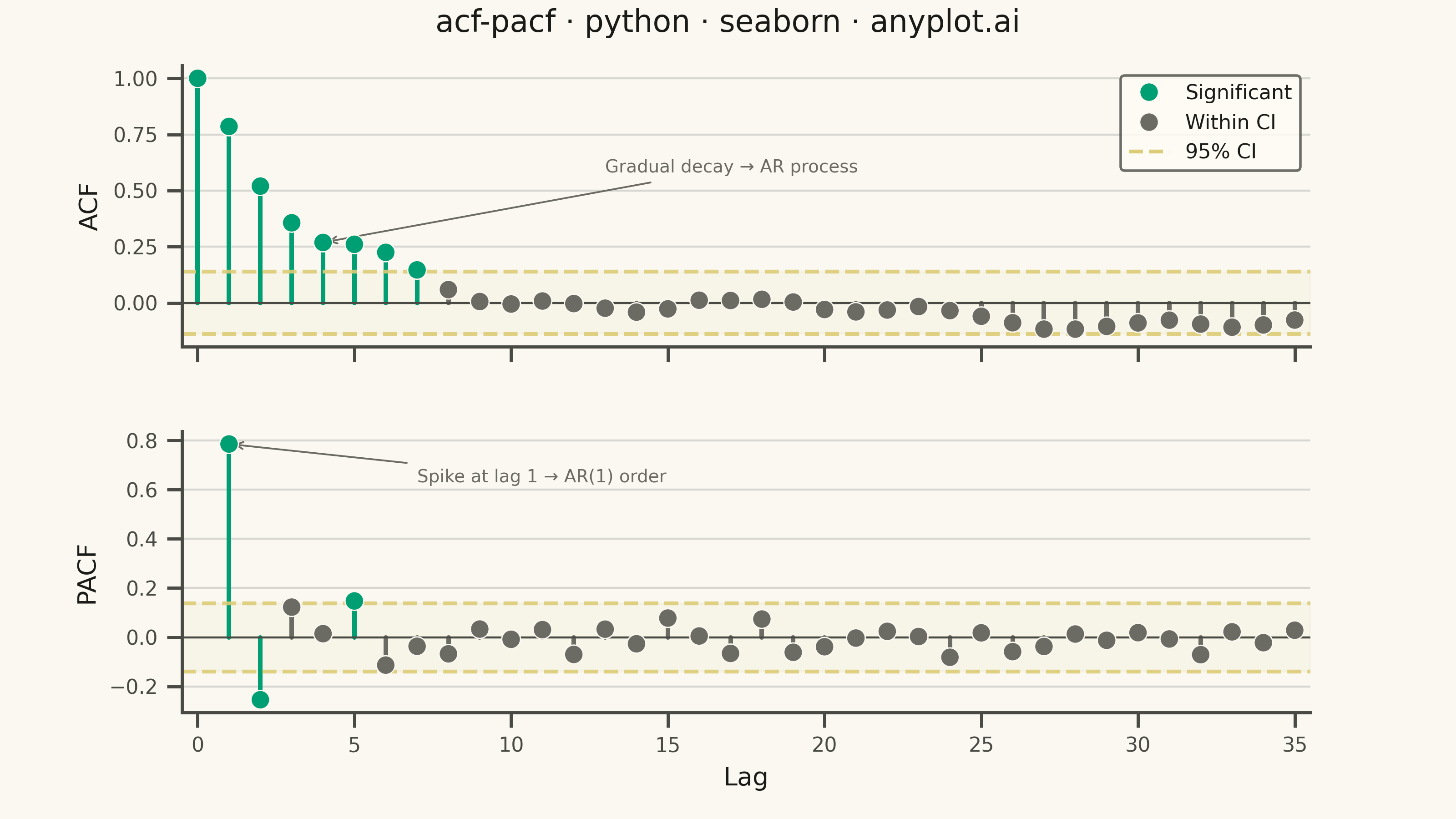
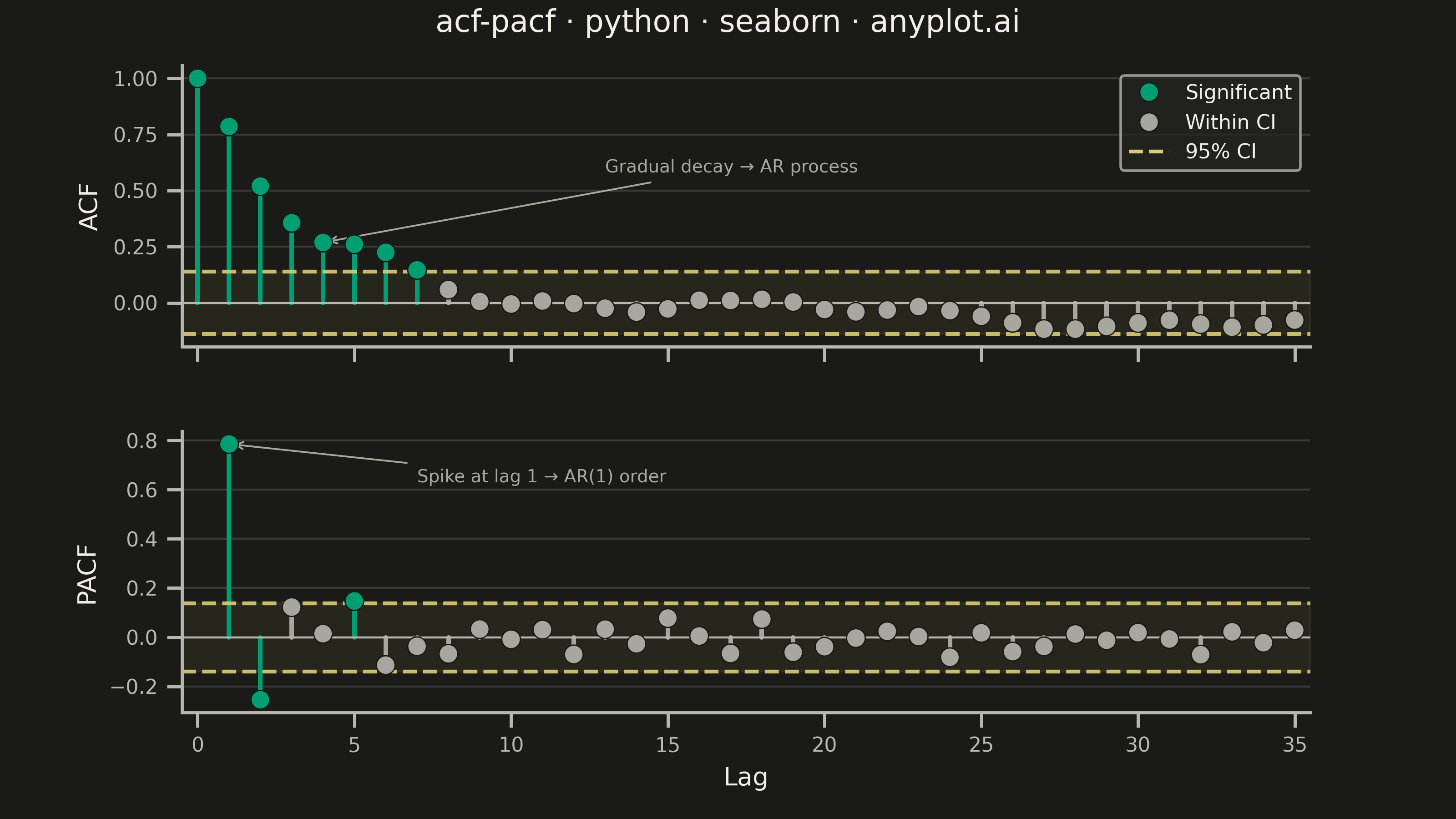
Displays the autocorrelation function (ACF) and partial autocorrelation function (PACF) of a time series as vertical stem/bar plots arranged in two vertically stacked subplots. Each lag is represented by a vertical line from zero to the correlation value, with horizontal dashed lines indicating 95% confidence bounds. These plots are essential for identifying the order of AR and MA components in ARIMA modeling and for diagnosing residual independence.
""" anyplot.ai
acf-pacf: Autocorrelation and Partial Autocorrelation (ACF/PACF) Plot
Library: seaborn 0.13.2 | Python 3.13.13
Quality: 88/100 | Updated: 2026-06-10
"""

import os
import sys


# Prevent local files (matplotlib.py, etc.) from shadowing installed packages
_script_dir = os.path.dirname(os.path.abspath(__file__))
if _script_dir in sys.path:
    sys.path.remove(_script_dir)
if "" in sys.path:
    sys.path.remove("")
if "." in sys.path:
    sys.path.remove(".")

import matplotlib.pyplot as plt
import numpy as np
import pandas as pd
import seaborn as sns


# Theme tokens (Imprint chrome — see prompts/default-style-guide.md)
THEME = os.getenv("ANYPLOT_THEME", "light")
PAGE_BG = "#FAF8F1" if THEME == "light" else "#1A1A17"
ELEVATED_BG = "#FFFDF6" if THEME == "light" else "#242420"
INK = "#1A1A17" if THEME == "light" else "#F0EFE8"
INK_SOFT = "#4A4A44" if THEME == "light" else "#B8B7B0"
INK_MUTED = "#6B6A63" if THEME == "light" else "#A8A79F"

BRAND = "#009E73"  # Imprint palette position 1 — always first series
ANYPLOT_AMBER = "#DDCC77"  # caution/threshold marker for CI bounds

sns.set_theme(
    style="ticks",
    rc={
        "figure.facecolor": PAGE_BG,
        "axes.facecolor": PAGE_BG,
        "axes.edgecolor": INK_SOFT,
        "axes.labelcolor": INK,
        "text.color": INK,
        "xtick.color": INK_SOFT,
        "ytick.color": INK_SOFT,
        "grid.color": INK,
        "grid.alpha": 0.15,
        "legend.facecolor": ELEVATED_BG,
        "legend.edgecolor": INK_SOFT,
    },
)

# Data: ARMA(1,1) process with seasonal component (airline passenger residuals)
np.random.seed(42)
n_obs = 200
ar1_coeff = 0.7
ma1_coeff = 0.4
seasonal_period = 12
seasonal_strength = 0.3
noise = np.random.randn(n_obs)
series = np.zeros(n_obs)
series[0] = noise[0]
for t in range(1, n_obs):
    seasonal = seasonal_strength * np.sin(2 * np.pi * t / seasonal_period)
    series[t] = ar1_coeff * series[t - 1] + noise[t] + ma1_coeff * noise[t - 1] + seasonal

# Compute ACF
n_lags = 35
mean = np.mean(series)
var = np.sum((series - mean) ** 2)
acf_values = np.array([np.sum((series[: n_obs - k] - mean) * (series[k:] - mean)) / var for k in range(n_lags + 1)])

# Compute PACF via Durbin-Levinson recursion
pacf_values = np.zeros(n_lags + 1)
pacf_values[0] = 1.0
pacf_values[1] = acf_values[1]
phi = np.zeros((n_lags + 1, n_lags + 1))
phi[1, 1] = acf_values[1]
for k in range(2, n_lags + 1):
    num = acf_values[k] - np.sum(phi[k - 1, 1:k] * acf_values[k - 1 : 0 : -1])
    den = 1.0 - np.sum(phi[k - 1, 1:k] * acf_values[1:k])
    phi[k, k] = num / den if den != 0 else 0
    for j in range(1, k):
        phi[k, j] = phi[k - 1, j] - phi[k, k] * phi[k - 1, k - j]
    pacf_values[k] = phi[k, k]

lags_acf = np.arange(0, n_lags + 1)
lags_pacf = np.arange(1, n_lags + 1)
conf_bound = 1.96 / np.sqrt(n_obs)

# DataFrames with significance classification for seaborn hue encoding
acf_df = pd.DataFrame(
    {
        "Lag": lags_acf,
        "Correlation": acf_values,
        "Significance": np.where((np.abs(acf_values) > conf_bound) | (lags_acf == 0), "Significant", "Within CI"),
    }
)
pacf_df = pd.DataFrame(
    {
        "Lag": lags_pacf,
        "Correlation": pacf_values[1:],
        "Significance": np.where(np.abs(pacf_values[1:]) > conf_bound, "Significant", "Within CI"),
    }
)

sig_palette = {"Significant": BRAND, "Within CI": INK_MUTED}


def make_stem_df(df):
    # Paired-row format required by sns.lineplot(units='Lag') to draw each stem as an
    # individual vertical segment without cross-lag interpolation.
    rows = []
    for _, row in df.iterrows():
        rows.append({"Lag": row["Lag"], "y": 0.0, "Significance": row["Significance"]})
        rows.append({"Lag": row["Lag"], "y": row["Correlation"], "Significance": row["Significance"]})
    return pd.DataFrame(rows)


acf_stem_df = make_stem_df(acf_df)
pacf_stem_df = make_stem_df(pacf_df)

# Canvas: figsize=(8, 4.5) @ dpi=400 → exactly 3200×1800 px (landscape 16:9)
fig, (ax_acf, ax_pacf) = plt.subplots(2, 1, figsize=(8, 4.5), dpi=400, facecolor=PAGE_BG, sharex=True)
ax_acf.set_facecolor(PAGE_BG)
ax_pacf.set_facecolor(PAGE_BG)

# ACF: sns.lineplot with units='Lag' draws each significance-colored stem as a
# discrete vertical segment — idiomatic seaborn statistical unit rendering
sns.lineplot(
    data=acf_stem_df,
    x="Lag",
    y="y",
    hue="Significance",
    palette=sig_palette,
    units="Lag",
    estimator=None,
    linewidth=1.8,
    ax=ax_acf,
    legend=False,
)
sns.scatterplot(
    data=acf_df,
    x="Lag",
    y="Correlation",
    hue="Significance",
    hue_order=["Significant", "Within CI"],
    palette=sig_palette,
    s=55,
    zorder=5,
    edgecolor=PAGE_BG,
    linewidth=0.5,
    ax=ax_acf,
    legend=True,
)

# PACF: same seaborn approach from lag 1
sns.lineplot(
    data=pacf_stem_df,
    x="Lag",
    y="y",
    hue="Significance",
    palette=sig_palette,
    units="Lag",
    estimator=None,
    linewidth=1.8,
    ax=ax_pacf,
    legend=False,
)
sns.scatterplot(
    data=pacf_df,
    x="Lag",
    y="Correlation",
    hue="Significance",
    palette=sig_palette,
    s=55,
    zorder=5,
    edgecolor=PAGE_BG,
    linewidth=0.5,
    ax=ax_pacf,
    legend=False,
)

# CI bounds, baseline, and grid for both panels
for ax in (ax_acf, ax_pacf):
    ax.axhline(y=0, color=INK_SOFT, linewidth=0.8)
    ax.axhline(y=conf_bound, color=ANYPLOT_AMBER, linestyle="--", linewidth=1.5, alpha=0.9)
    ax.axhline(y=-conf_bound, color=ANYPLOT_AMBER, linestyle="--", linewidth=1.5, alpha=0.9)
    ax.fill_between([-0.5, n_lags + 0.5], -conf_bound, conf_bound, color=ANYPLOT_AMBER, alpha=0.07)
    ax.set_xlim(-0.5, n_lags + 0.5)
    ax.yaxis.grid(True, alpha=0.15, linewidth=0.8, color=INK)
    ax.tick_params(axis="both", labelsize=8, colors=INK_SOFT)

# Spine styling
sns.despine(fig=fig)
for ax in (ax_acf, ax_pacf):
    ax.spines["left"].set_color(INK_SOFT)
    ax.spines["bottom"].set_color(INK_SOFT)

# Axis labels
ax_acf.set_ylabel("ACF", fontsize=10, color=INK)
ax_pacf.set_ylabel("PACF", fontsize=10, color=INK)
ax_pacf.set_xlabel("Lag", fontsize=10, color=INK)

# X-ticks every 5 lags (shared axis — set once on either panel)
ax_pacf.set_xticks(np.arange(0, n_lags + 1, 5))

# Legend in ACF panel: seaborn auto-generates Significant/Within CI handles from
# scatterplot hue; extend with the amber CI dashed-line handle
handles, labels = ax_acf.get_legend_handles_labels()
ci_handle = plt.Line2D([0], [0], linestyle="--", color=ANYPLOT_AMBER, linewidth=1.5)
handles.append(ci_handle)
labels.append("95% CI")
ax_acf.legend(handles=handles, labels=labels, loc="upper right", fontsize=8, facecolor=ELEVATED_BG, edgecolor=INK_SOFT)

# Data storytelling annotations — AR(1) signature visible in both panels
ax_acf.annotate(
    "Gradual decay → AR process",
    xy=(4, acf_values[4]),
    xytext=(13, 0.58),
    fontsize=7,
    color=INK_MUTED,
    arrowprops={"arrowstyle": "->", "color": INK_MUTED, "lw": 0.7},
)
ax_pacf.annotate(
    "Spike at lag 1 → AR(1) order",
    xy=(1, pacf_values[1]),
    xytext=(7, 0.63),
    fontsize=7,
    color=INK_MUTED,
    arrowprops={"arrowstyle": "->", "color": INK_MUTED, "lw": 0.7},
)

# Title — "acf-pacf · python · seaborn · anyplot.ai" is 40 chars (< 67 baseline → fontsize=12)
title = "acf-pacf · python · seaborn · anyplot.ai"
fig.suptitle(title, fontsize=12, fontweight="medium", color=INK, y=0.99)
fig.subplots_adjust(top=0.92, bottom=0.13, hspace=0.3)

# Save — no bbox_inches to preserve exact 3200×1800 canvas
plt.savefig(f"plot-{THEME}.png", dpi=400, facecolor=PAGE_BG)
Runnable source as JSON, for any HTTP client: https://api.anyplot.ai/specs/acf-pacf/seaborn/code. Any spec id and library id listed in llms-full.txt fit the same URL shape; every URL below is complete and callable.
{
  "spec_id": "acf-pacf",
  "language": "python",
  "library": "seaborn",
  "page": "https://anyplot.ai/acf-pacf/python/seaborn",
  "hub": "https://anyplot.ai/acf-pacf",
  "code_json": "https://api.anyplot.ai/specs/acf-pacf/seaborn/code",
  "spec_json": "https://api.anyplot.ai/specs/acf-pacf",
  "render_light_png": "https://storage.googleapis.com/anyplot-images/plots/acf-pacf/python/seaborn/plot-light.png",
  "render_dark_png": "https://storage.googleapis.com/anyplot-images/plots/acf-pacf/python/seaborn/plot-dark.png",
  "quality_score": 88.0,
  "license": "MIT",
  "guide": "https://anyplot.ai/llms.txt"
}
Part of Autocorrelation and Partial Autocorrelation (ACF/PACF) Plot on anyplot.ai.