The same plot in 13 other libraries — Python: Altair, Bokeh, lets-plot, Matplotlib, Plotly, plotnine, Pygal, Seaborn; Julia: Makie.jl; JavaScript: D3.js, Apache ECharts, Highcharts, MUI X Charts. Compare all 14 side by side: Opinion Flow Diagram in Python, R, Julia and JavaScript.
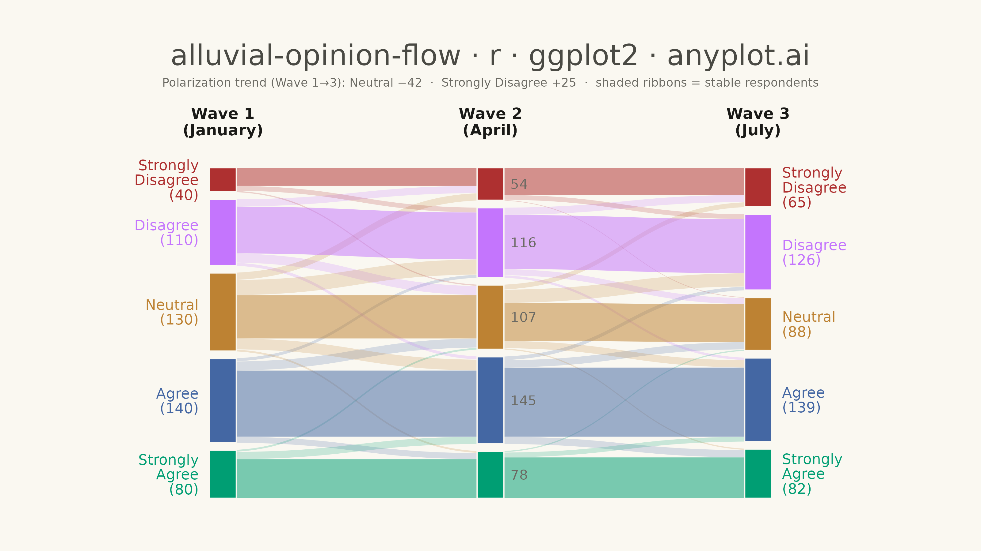
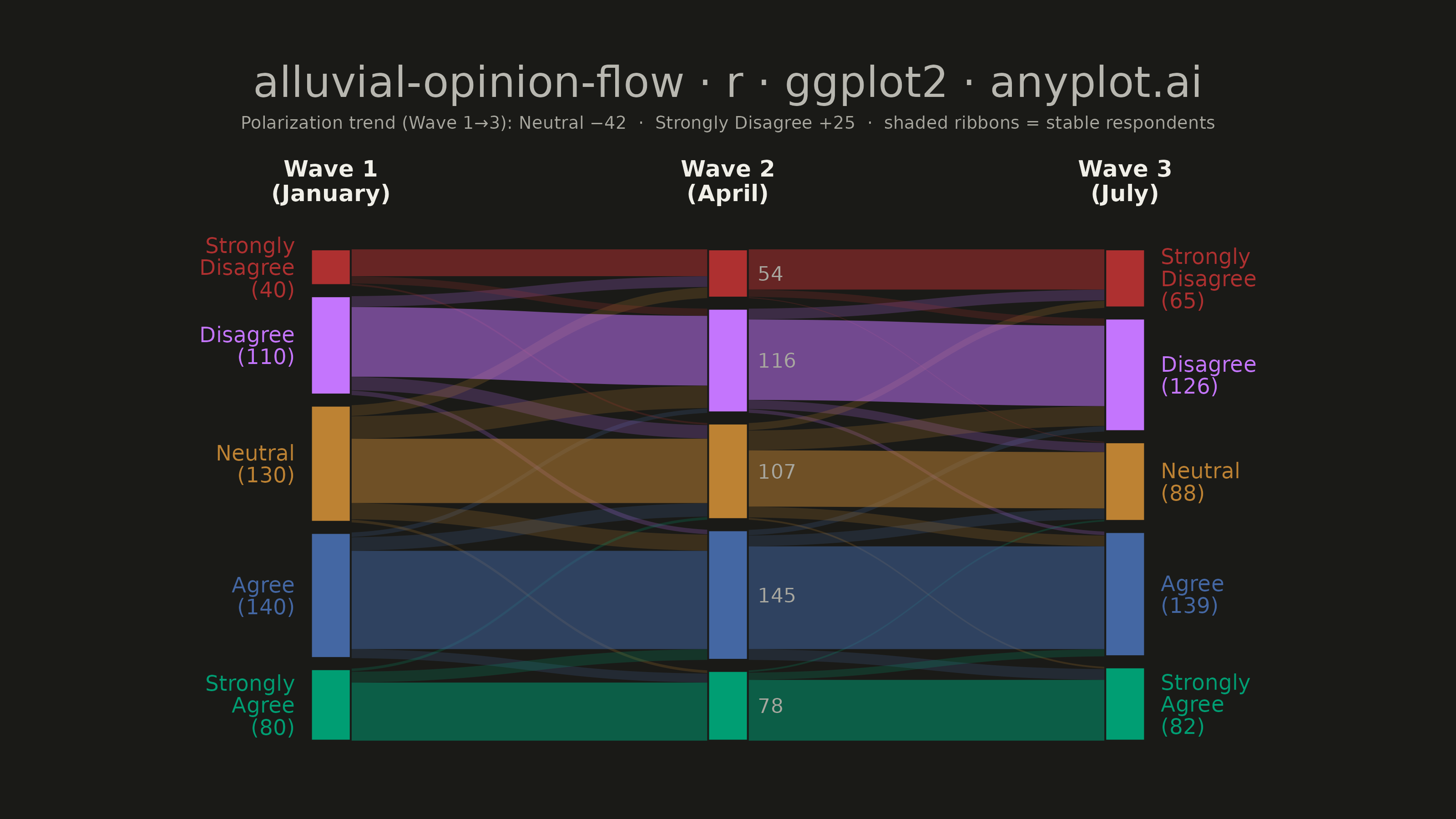
An alluvial/Sankey-style diagram showing how opinions or group memberships shift between survey waves or time periods. Flows connect the same response categories across columns, revealing patterns of opinion change, stability, and polarization. Unlike a basic alluvial diagram, this variant emphasizes distinguishing stable respondents from net changers and displays respondent totals per category at each wave.
#' anyplot.ai
#' alluvial-opinion-flow: Opinion Flow Diagram
#' Library: ggplot2 3.5.1 | R 4.4.1
#' Quality: 88/100 | Created: 2026-05-30

library(ggplot2)
library(ragg)

set.seed(42)

# Theme tokens (Imprint palette, theme-adaptive chrome)
THEME       <- Sys.getenv("ANYPLOT_THEME", "light")
PAGE_BG     <- if (THEME == "light") "#FAF8F1" else "#1A1A17"
ELEVATED_BG <- if (THEME == "light") "#FFFDF6" else "#242420"
INK         <- if (THEME == "light") "#1A1A17" else "#F0EFE8"
INK_SOFT    <- if (THEME == "light") "#4A4A44" else "#B8B7B0"
INK_MUTED   <- if (THEME == "light") "#6B6A63" else "#A8A79F"

# Imprint palette — semantic mapping: positive→green, neutral→ochre, negative→red
IMPRINT_PALETTE <- c(
    "Strongly Agree"    = "#009E73",   # brand green (positive)
    "Agree"             = "#4467A3",   # blue
    "Neutral"           = "#BD8233",   # ochre
    "Disagree"          = "#C475FD",   # lavender
    "Strongly Disagree" = "#AE3030"    # matte red (negative)
)

categories <- names(IMPRINT_PALETTE)

# Climate policy opinion survey: 500 respondents tracked across 3 quarterly waves
# Transition matrices show increasing polarization over time
m12 <- matrix(c(
    65, 12,  3,  0,  0,   # Strongly Agree →
    10,110, 15,  5,  0,   # Agree →
     3, 18, 72, 25, 12,   # Neutral →
     0,  5, 15, 78, 12,   # Disagree →
     0,  0,  2,  8, 30    # Strongly Disagree →
), nrow = 5, byrow = TRUE, dimnames = list(categories, categories))

m23 <- matrix(c(
    68,  8,  2,  0,  0,   # Strongly Agree →
    12,115, 12,  6,  0,   # Agree →
     2, 12, 63, 22,  8,   # Neutral →
     0,  4, 10, 90, 12,   # Disagree →
     0,  0,  1,  8, 45    # Strongly Disagree →
), nrow = 5, byrow = TRUE, dimnames = list(categories, categories))

wave_x  <- c(1.0, 2.0, 3.0)
node_w  <- 0.10

# Compute stacked y-positions for each category at a wave
stack_pos <- function(totals, gap_frac = 0.025) {
    g   <- sum(totals) * gap_frac
    pos <- data.frame(
        category = names(totals), total = as.numeric(totals),
        y_bot = NA_real_, y_top = NA_real_, y_mid = NA_real_,
        stringsAsFactors = FALSE
    )
    y <- 0
    for (i in seq_len(nrow(pos))) {
        pos$y_bot[i] <- y
        pos$y_top[i] <- y + pos$total[i]
        pos$y_mid[i] <- y + pos$total[i] / 2
        y            <- y + pos$total[i] + g
    }
    pos
}

pos1 <- stack_pos(setNames(rowSums(m12), categories))
pos2 <- stack_pos(setNames(colSums(m12), categories))
pos3 <- stack_pos(setNames(colSums(m23), categories))

# Compute flow y-segments — stacked within each node in category order
flow_segs <- function(mat, pfrom, pto) {
    src_off <- setNames(pfrom$y_bot, pfrom$category)
    tgt_off <- setNames(pto$y_bot,   pto$category)
    rows    <- list()
    for (from_c in categories) {
        for (to_c in categories) {
            cnt <- mat[from_c, to_c]
            if (cnt == 0) next
            y1b <- src_off[[from_c]]
            y2b <- tgt_off[[to_c]]
            rows[[length(rows) + 1]] <- data.frame(
                from = from_c, to = to_c, count = cnt,
                y1_bot = y1b, y1_top = y1b + cnt,
                y2_bot = y2b, y2_top = y2b + cnt,
                stringsAsFactors = FALSE
            )
            src_off[[from_c]] <- src_off[[from_c]] + cnt
            tgt_off[[to_c]]   <- tgt_off[[to_c]]   + cnt
        }
    }
    do.call(rbind, rows)
}

segs12 <- flow_segs(m12, pos1, pos2)
segs23 <- flow_segs(m23, pos2, pos3)

# S-curve bezier ribbon polygon (control points keep curve horizontal at nodes)
bezier_ribbon <- function(x1, x2, y1b, y1t, y2b, y2t, n = 80) {
    t  <- seq(0, 1, length.out = n)
    xm <- (x1 + x2) / 2
    bx <- (1 - t)^3 * x1 + 3 * (1 - t)^2 * t * xm + 3 * (1 - t) * t^2 * xm + t^3 * x2
    yh <- (1 - t)^3 * y1t + 3 * (1 - t)^2 * t * y1t + 3 * (1 - t) * t^2 * y2t + t^3 * y2t
    yl <- (1 - t)^3 * y1b + 3 * (1 - t)^2 * t * y1b + 3 * (1 - t) * t^2 * y2b + t^3 * y2b
    data.frame(x = c(bx, rev(bx)), y = c(yh, rev(yl)))
}

make_ribbons <- function(segs, x1, x2) {
    do.call(rbind, lapply(seq_len(nrow(segs)), function(i) {
        s   <- segs[i, ]
        rbn <- bezier_ribbon(x1, x2, s$y1_bot, s$y1_top, s$y2_bot, s$y2_top)
        rbn$from      <- s$from
        rbn$is_stable <- s$from == s$to
        rbn$ribbon_id <- paste0(s$from, "_", s$to, "_x", x1)
        rbn
    }))
}

ribbons <- rbind(
    make_ribbons(segs12, wave_x[1], wave_x[2]),
    make_ribbons(segs23, wave_x[2], wave_x[3])
)

# Split stable (same category) vs. changer ribbons for distinct visual treatment
ribbons_changers <- ribbons[!ribbons$is_stable, ]
ribbons_stable   <- ribbons[ribbons$is_stable,  ]

# Node rectangles for all 3 waves
node_rects <- do.call(rbind, lapply(list(
    list(pos = pos1, wx = wave_x[1]),
    list(pos = pos2, wx = wave_x[2]),
    list(pos = pos3, wx = wave_x[3])
), function(pw) {
    data.frame(
        category = pw$pos$category,
        xmin  = pw$wx - node_w / 2,
        xmax  = pw$wx + node_w / 2,
        ymin  = pw$pos$y_bot,
        ymax  = pw$pos$y_top,
        y_mid = pw$pos$y_mid,
        x_ctr = pw$wx,
        total = pw$pos$total,
        stringsAsFactors = FALSE
    )
}))

# Wave column headers
wave_top <- max(pos1$y_top, pos2$y_top, pos3$y_top)
headers <- data.frame(
    x     = wave_x,
    y     = wave_top * 1.14,
    label = c("Wave 1\n(January)", "Wave 2\n(April)", "Wave 3\n(July)")
)

# Category + count labels: left of Wave 1 nodes, right of Wave 3 nodes
wrap_cat <- function(cat) gsub("Strongly ", "Strongly\n", cat)

cat_left <- data.frame(
    x        = wave_x[1] - node_w / 2 - 0.04,
    y        = pos1$y_mid,
    label    = paste0(wrap_cat(pos1$category), "\n(", pos1$total, ")"),
    category = pos1$category,
    hjust    = 1.0,
    stringsAsFactors = FALSE
)
cat_right <- data.frame(
    x        = wave_x[3] + node_w / 2 + 0.04,
    y        = pos3$y_mid,
    label    = paste0(wrap_cat(pos3$category), "\n(", pos3$total, ")"),
    category = pos3$category,
    hjust    = 0.0,
    stringsAsFactors = FALSE
)

# Wave 2 count labels (right side of Wave 2 nodes)
w2_counts <- data.frame(
    x     = wave_x[2] + node_w / 2 + 0.025,
    y     = pos2$y_mid,
    label = as.character(pos2$total),
    hjust = 0.0
)

# Net change Wave 1 → Wave 3 for polarization subtitle
w1_totals  <- setNames(pos1$total, pos1$category)
w3_totals  <- setNames(pos3$total, pos3$category)

# Title: scale fontsize for long title string
title_str    <- "alluvial-opinion-flow · r · ggplot2 · anyplot.ai"
title_fs     <- max(8L, round(12L * 67L / nchar(title_str)))
subtitle_str <- paste0(
    "Polarization trend (Wave 1→3): Neutral −42  ·  ",
    "Strongly Disagree +25  ·  shaded ribbons = stable respondents"
)

p <- ggplot() +
    # Changer ribbons (cross-category flows) drawn first at lower opacity
    geom_polygon(
        data  = ribbons_changers,
        aes(x = x, y = y, group = ribbon_id, fill = from),
        alpha = 0.20,
        color = NA
    ) +
    # Stable (same-category) ribbons emphasized with higher opacity
    geom_polygon(
        data  = ribbons_stable,
        aes(x = x, y = y, group = ribbon_id, fill = from),
        alpha = 0.52,
        color = NA
    ) +
    # Nodes
    geom_rect(
        data      = node_rects,
        aes(xmin = xmin, xmax = xmax, ymin = ymin, ymax = ymax, fill = category),
        color     = PAGE_BG,
        linewidth = 0.35
    ) +
    # Category + count labels (Wave 1 left, Wave 3 right)
    geom_text(
        data     = cat_left,
        aes(x = x, y = y, label = label, hjust = hjust, color = category),
        size     = 3.0,
        lineheight = 0.85
    ) +
    geom_text(
        data     = cat_right,
        aes(x = x, y = y, label = label, hjust = hjust, color = category),
        size     = 3.0,
        lineheight = 0.85
    ) +
    # Wave 2 count labels
    geom_text(
        data  = w2_counts,
        aes(x = x, y = y, label = label, hjust = hjust),
        size  = 2.8,
        color = INK_MUTED
    ) +
    # Wave headers
    geom_text(
        data     = headers,
        aes(x = x, y = y, label = label),
        size     = 3.2,
        color    = INK,
        fontface = "bold",
        lineheight = 0.9
    ) +
    scale_fill_manual(values  = IMPRINT_PALETTE, guide = "none") +
    scale_color_manual(values = IMPRINT_PALETTE, guide = "none") +
    labs(title = title_str, subtitle = subtitle_str) +
    theme_void() +
    theme(
        plot.background = element_rect(fill = PAGE_BG, color = NA),
        plot.title      = element_text(
            color  = INK_SOFT,
            size   = title_fs,
            hjust  = 0.5,
            margin = margin(t = 14, b = 4)
        ),
        plot.subtitle   = element_text(
            color  = INK_MUTED,
            size   = 7,
            hjust  = 0.5,
            margin = margin(b = 8)
        ),
        plot.margin = margin(t = 12, r = 100, b = 20, l = 100, unit = "pt")
    ) +
    coord_cartesian(clip = "off")

ggsave(
    filename = sprintf("plot-%s.png", THEME),
    plot     = p,
    device   = ragg::agg_png,
    width    = 8,
    height   = 4.5,
    units    = "in",
    dpi      = 400
)
Runnable source as JSON, for any HTTP client: https://api.anyplot.ai/specs/alluvial-opinion-flow/ggplot2/code. Any spec id and library id listed in llms-full.txt fit the same URL shape; every URL below is complete and callable.
{
  "spec_id": "alluvial-opinion-flow",
  "language": "r",
  "library": "ggplot2",
  "page": "https://anyplot.ai/alluvial-opinion-flow/r/ggplot2",
  "hub": "https://anyplot.ai/alluvial-opinion-flow",
  "code_json": "https://api.anyplot.ai/specs/alluvial-opinion-flow/ggplot2/code",
  "spec_json": "https://api.anyplot.ai/specs/alluvial-opinion-flow",
  "render_light_png": "https://storage.googleapis.com/anyplot-images/plots/alluvial-opinion-flow/r/ggplot2/plot-light.png",
  "render_dark_png": "https://storage.googleapis.com/anyplot-images/plots/alluvial-opinion-flow/r/ggplot2/plot-dark.png",
  "quality_score": 88.0,
  "license": "MIT",
  "guide": "https://anyplot.ai/llms.txt"
}
Part of Opinion Flow Diagram on anyplot.ai.