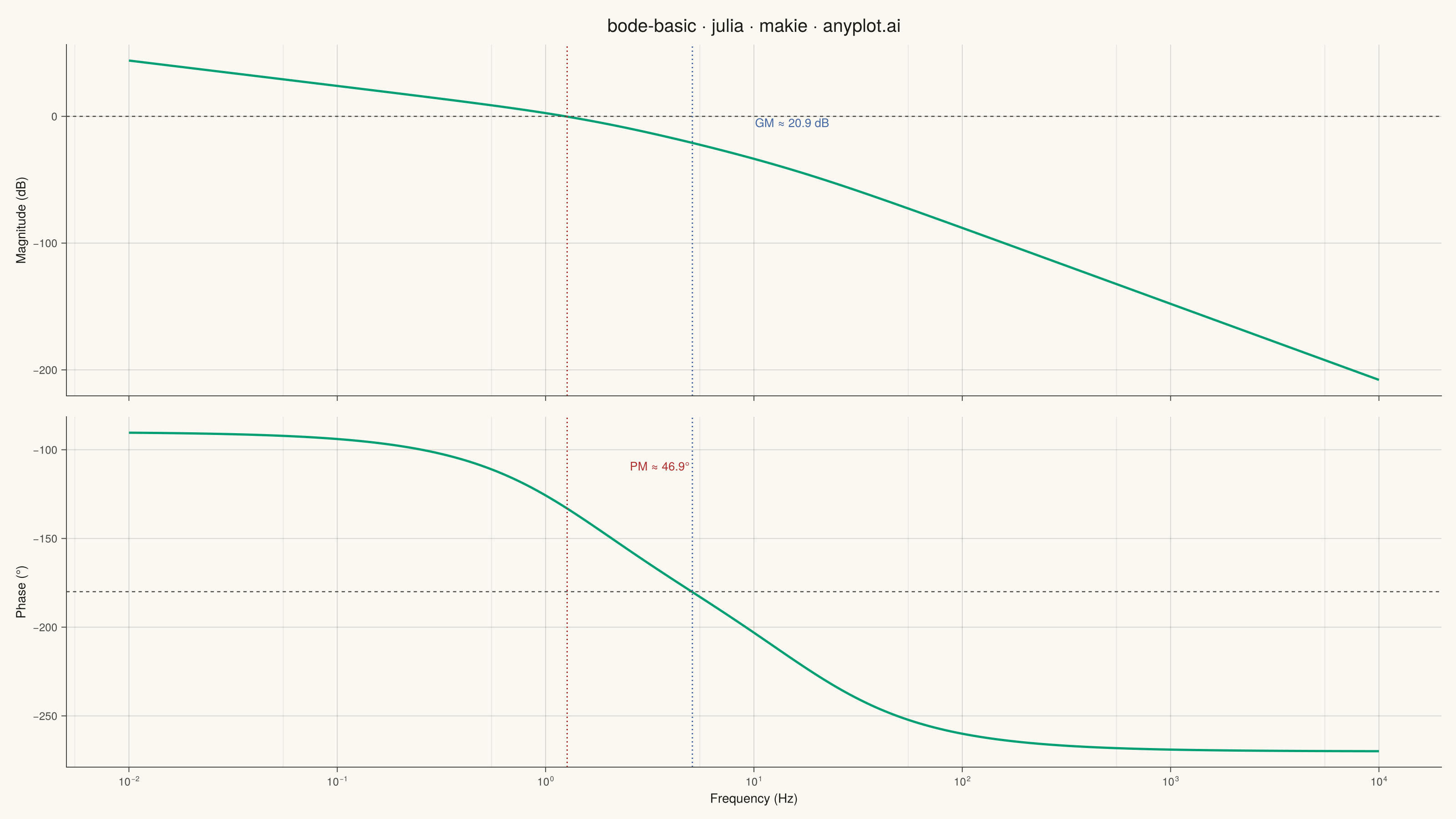
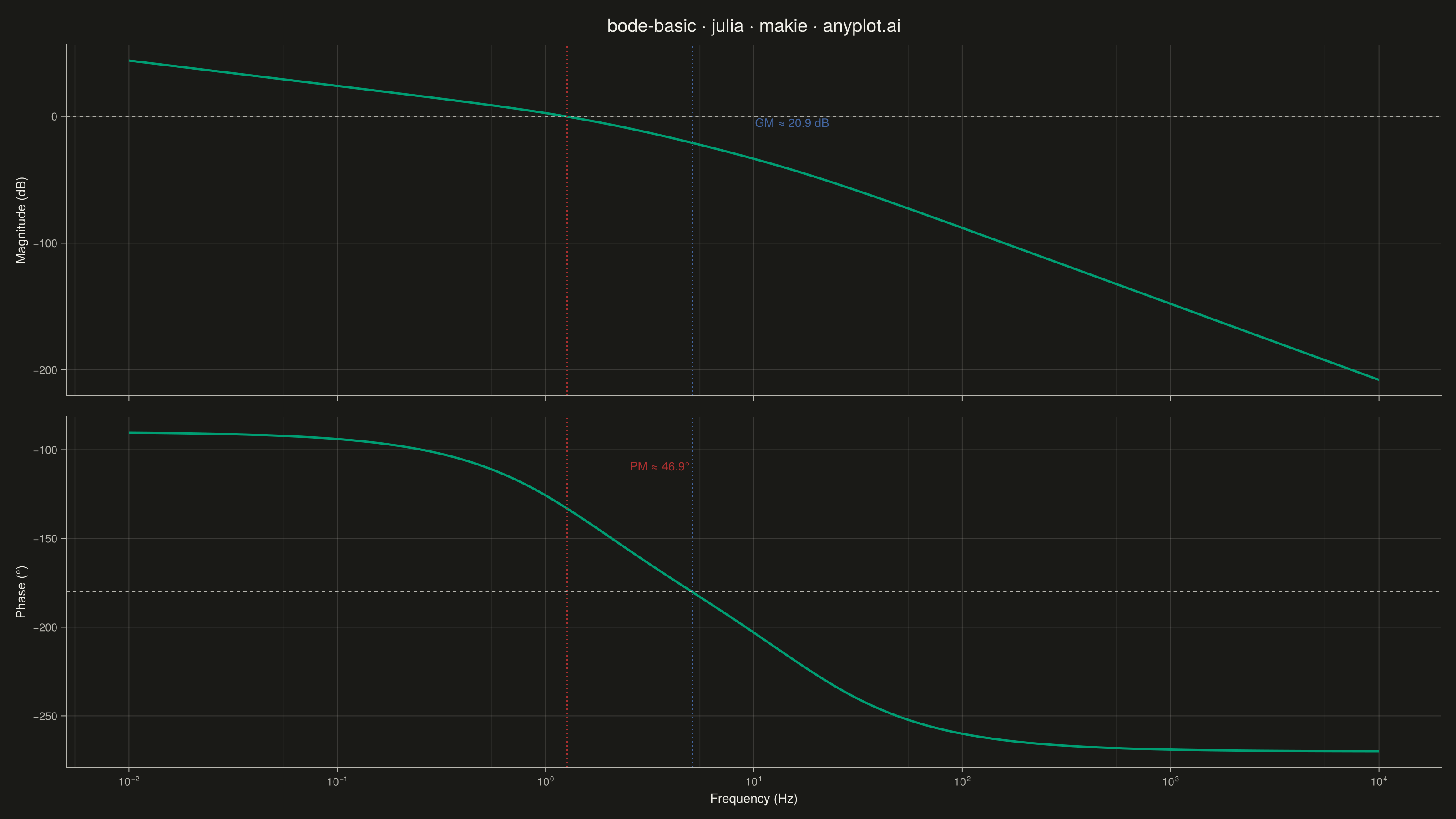
A Bode plot displays a system's frequency response as two vertically aligned panels: magnitude (in decibels) on top and phase (in degrees) on the bottom, both plotted against frequency on a shared logarithmic scale. This visualization is fundamental in control systems engineering and signal processing for analyzing how a system responds to sinusoidal inputs across a range of frequencies, revealing stability characteristics, bandwidth, and resonance behavior.
# anyplot.ai
# bode-basic: Bode Plot for Frequency Response
# Library: makie 0.22.10 | Julia 1.11.9
# Quality: 89/100 | Created: 2026-06-17

using CairoMakie
using Colors

# Theme tokens
const THEME    = get(ENV, "ANYPLOT_THEME", "light")
const PAGE_BG  = THEME == "light" ? colorant"#FAF8F1" : colorant"#1A1A17"
const INK      = THEME == "light" ? colorant"#1A1A17" : colorant"#F0EFE8"
const INK_SOFT = THEME == "light" ? colorant"#4A4A44" : colorant"#B8B7B0"

const IMPRINT = [
    colorant"#009E73",  # 1 — brand green (first series)
    colorant"#C475FD",  # 2 — lavender
    colorant"#4467A3",  # 3 — blue
    colorant"#BD8233",  # 4 — ochre
    colorant"#AE3030",  # 5 — matte red
    colorant"#2ABCCD",  # 6 — cyan
    colorant"#954477",  # 7 — rose
    colorant"#99B314",  # 8 — lime
]

# Data — open-loop transfer function: H(s) = K / (s(τ₁s+1)(τ₂s+1))
# Type-1 third-order system; phase crosses -180° at ω_pc = 1/√(τ₁τ₂)
const K_gain = 10.0
const τ₁     = 0.1    # primary lag, s
const τ₂     = 0.01   # secondary lag, s

freq_hz = 10.0 .^ range(-2.0, 4.0; length = 600)  # 0.01–10000 Hz per spec
ω = 2π .* freq_hz                                   # rad/s for transfer function

magnitude_db = 20.0 .* log10.(
    K_gain ./ (ω .* sqrt.(1.0 .+ (τ₁ .* ω).^2) .* sqrt.(1.0 .+ (τ₂ .* ω).^2))
)
phase_deg = -90.0 .- rad2deg.(atan.(τ₁ .* ω)) .- rad2deg.(atan.(τ₂ .* ω))

# Stability margins
pc_idx     = findfirst(phase_deg .<= -180.0)
gc_idx     = findfirst(magnitude_db .<= 0.0)
gm_db      = isnothing(pc_idx) ? Inf : -magnitude_db[pc_idx]
pm_deg_val = isnothing(gc_idx) ? Inf : 180.0 + phase_deg[gc_idx]

# Figure
fig = Figure(
    size            = (1600, 900),
    fontsize        = 14,
    backgroundcolor = PAGE_BG,
)

axis_style = (
    backgroundcolor    = PAGE_BG,
    topspinevisible    = false,
    rightspinevisible  = false,
    leftspinecolor     = INK_SOFT,
    bottomspinecolor   = INK_SOFT,
    xtickcolor         = INK_SOFT,
    ytickcolor         = INK_SOFT,
    xticklabelcolor    = INK_SOFT,
    yticklabelcolor    = INK_SOFT,
    xlabelcolor        = INK,
    ylabelcolor        = INK,
    xticklabelsize     = 12,
    yticklabelsize     = 12,
    xlabelsize         = 14,
    ylabelsize         = 14,
    xscale             = log10,
    xgridcolor         = RGBAf(INK.r, INK.g, INK.b, 0.15f0),
    ygridcolor         = RGBAf(INK.r, INK.g, INK.b, 0.15f0),
    xgridvisible       = true,
    ygridvisible       = true,
    xminorgridvisible  = true,
    yminorgridvisible  = false,
    xminorgridcolor    = RGBAf(INK.r, INK.g, INK.b, 0.07f0),
)

ax_mag = Axis(fig[1, 1]; axis_style...,
    ylabel             = "Magnitude (dB)",
    xticklabelsvisible = false,
)

ax_phase = Axis(fig[2, 1]; axis_style...,
    xlabel = "Frequency (Hz)",
    ylabel = "Phase (°)",
)

linkxaxes!(ax_mag, ax_phase)

# Magnitude plot
lines!(ax_mag, freq_hz, magnitude_db; color = IMPRINT[1], linewidth = 2.5)
hlines!(ax_mag, [0.0]; color = INK_SOFT, linewidth = 1.2, linestyle = :dash)

# Phase plot
lines!(ax_phase, freq_hz, phase_deg; color = IMPRINT[1], linewidth = 2.5)
hlines!(ax_phase, [-180.0]; color = INK_SOFT, linewidth = 1.2, linestyle = :dash)

# Gain margin — phase crossover frequency (blue)
if !isnothing(pc_idx)
    vlines!(ax_mag,   [freq_hz[pc_idx]]; color = IMPRINT[3], linewidth = 1.5, linestyle = :dot)
    vlines!(ax_phase, [freq_hz[pc_idx]]; color = IMPRINT[3], linewidth = 1.5, linestyle = :dot)
    text!(ax_mag, freq_hz[pc_idx] * 2.0, magnitude_db[pc_idx] / 2.0;
        text     = "GM ≈ $(round(gm_db; digits = 1)) dB",
        color    = IMPRINT[3],
        fontsize = 13,
    )
end

# Phase margin — gain crossover frequency (matte red)
if !isnothing(gc_idx)
    vlines!(ax_mag,   [freq_hz[gc_idx]]; color = IMPRINT[5], linewidth = 1.5, linestyle = :dot)
    vlines!(ax_phase, [freq_hz[gc_idx]]; color = IMPRINT[5], linewidth = 1.5, linestyle = :dot)
    text!(ax_phase, freq_hz[gc_idx] * 2.0, phase_deg[gc_idx] + 20.0;
        text     = "PM ≈ $(round(pm_deg_val; digits = 1))°",
        color    = IMPRINT[5],
        fontsize = 13,
    )
end

# Figure-level title
Label(fig[0, 1], "bode-basic · julia · makie · anyplot.ai";
    fontsize  = 20,
    color     = INK,
    tellwidth = false,
)

rowgap!(fig.layout, 1, 10)

save(joinpath(@__DIR__, "plot-$(THEME).png"), fig; px_per_unit = 2)
Runnable source as JSON, for any HTTP client: https://api.anyplot.ai/specs/bode-basic/makie/code. Any spec id and library id listed in llms-full.txt fit the same URL shape; every URL below is complete and callable.
{
  "spec_id": "bode-basic",
  "language": "julia",
  "library": "makie",
  "page": "https://anyplot.ai/bode-basic/julia/makie",
  "hub": "https://anyplot.ai/bode-basic",
  "code_json": "https://api.anyplot.ai/specs/bode-basic/makie/code",
  "spec_json": "https://api.anyplot.ai/specs/bode-basic",
  "render_light_png": "https://storage.googleapis.com/anyplot-images/plots/bode-basic/julia/makie/plot-light.png",
  "render_dark_png": "https://storage.googleapis.com/anyplot-images/plots/bode-basic/julia/makie/plot-dark.png",
  "quality_score": 89.0,
  "license": "MIT",
  "guide": "https://anyplot.ai/llms.txt"
}
Part of Bode Plot for Frequency Response on anyplot.ai.