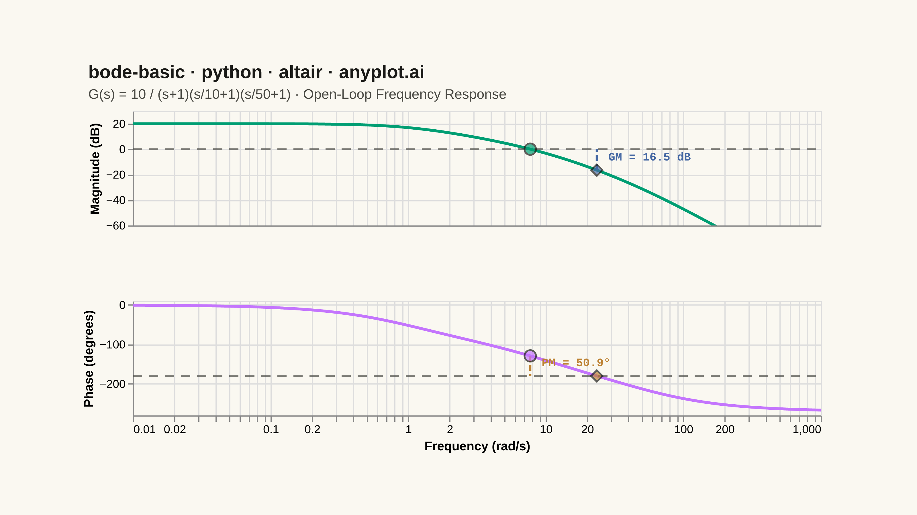
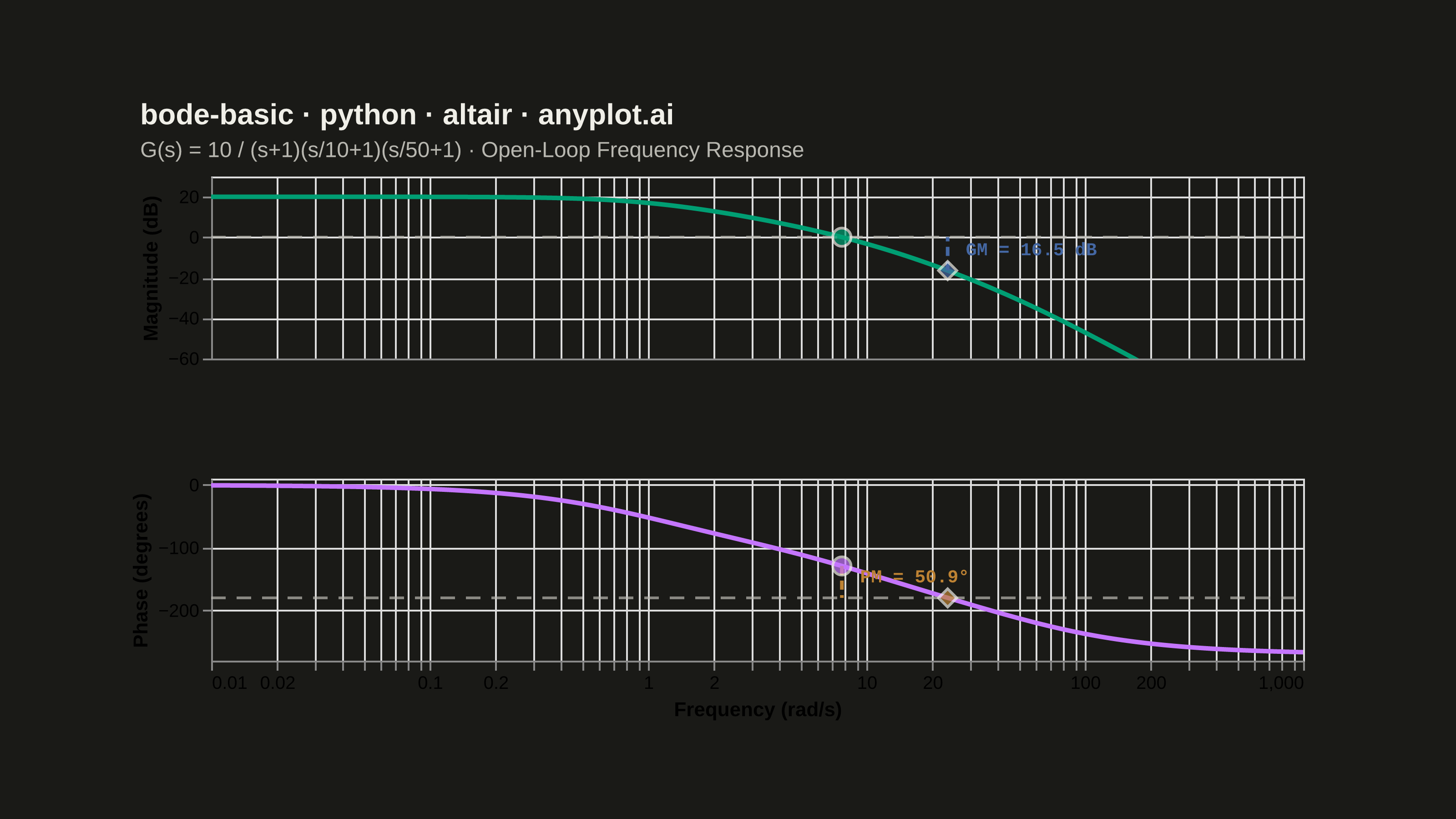
A Bode plot displays a system's frequency response as two vertically aligned panels: magnitude (in decibels) on top and phase (in degrees) on the bottom, both plotted against frequency on a shared logarithmic scale. This visualization is fundamental in control systems engineering and signal processing for analyzing how a system responds to sinusoidal inputs across a range of frequencies, revealing stability characteristics, bandwidth, and resonance behavior.
""" anyplot.ai
bode-basic: Bode Plot for Frequency Response
Library: altair 6.2.1 | Python 3.13.14
Quality: 91/100 | Updated: 2026-06-17
"""

import os
import sys


# Prevent self-import: 'python altair.py' adds this file's directory to
# sys.path[0], which would shadow the installed altair package.
_self_dir = os.path.dirname(os.path.abspath(__file__))
sys.path = [p for p in sys.path if os.path.realpath(p or os.getcwd()) != os.path.realpath(_self_dir)]
del _self_dir

import altair as alt
import numpy as np
import pandas as pd
from PIL import Image


THEME = os.getenv("ANYPLOT_THEME", "light")

# Theme-adaptive chrome tokens (Imprint)
PAGE_BG = "#FAF8F1" if THEME == "light" else "#1A1A17"
ELEVATED_BG = "#FFFDF6" if THEME == "light" else "#242420"
INK = "#1A1A17" if THEME == "light" else "#F0EFE8"
INK_SOFT = "#4A4A44" if THEME == "light" else "#B8B7B0"
INK_MUTED = "#6B6A63" if THEME == "light" else "#A8A79F"

# Imprint palette — first two series + annotation colors
CLR_MAG = "#009E73"  # Imprint[0] brand green — magnitude (first series)
CLR_PHASE = "#C475FD"  # Imprint[1] lavender — phase (second series)
CLR_GM = "#4467A3"  # Imprint[2] blue — gain margin annotation
CLR_PM = "#BD8233"  # Imprint[3] ochre — phase margin annotation

# Data — third-order open-loop transfer function:
# G(s) = 10 / (s+1)(s/10+1)(s/50+1); poles at -1, -10, -50; DC gain = 20 dB
omega = np.logspace(-2, 3, 600)
s = 1j * omega

K = 10.0
G = K / ((s / 1 + 1) * (s / 10 + 1) * (s / 50 + 1))

magnitude_db = 20 * np.log10(np.abs(G))
phase_deg = np.degrees(np.unwrap(np.angle(G)))

df = pd.DataFrame({"frequency": omega, "magnitude_db": magnitude_db, "phase_deg": phase_deg})

# Gain crossover frequency (|G| = 0 dB)
sign_changes_mag = np.where(np.diff(np.sign(magnitude_db)))[0]
gain_cross_idx = sign_changes_mag[0] if len(sign_changes_mag) > 0 else np.argmin(np.abs(magnitude_db))
gain_cross_freq = omega[gain_cross_idx]
gain_cross_phase = phase_deg[gain_cross_idx]
phase_margin = 180 + gain_cross_phase

# Phase crossover frequency (phase = -180°)
sign_changes_phase = np.where(np.diff(np.sign(phase_deg - (-180))))[0]
phase_cross_idx = sign_changes_phase[0] if len(sign_changes_phase) > 0 else np.argmin(np.abs(phase_deg + 180))
phase_cross_freq = omega[phase_cross_idx]
phase_cross_mag = magnitude_db[phase_cross_idx]
gain_margin = -phase_cross_mag

# Reference lines
ref_0db = pd.DataFrame({"x": [omega.min(), omega.max()], "y": [0, 0]})
ref_180 = pd.DataFrame({"x": [omega.min(), omega.max()], "y": [-180, -180]})

# Gain margin annotation (on magnitude panel)
gm_line = pd.DataFrame({"frequency": [phase_cross_freq, phase_cross_freq], "magnitude_db": [phase_cross_mag, 0]})
gm_label = pd.DataFrame(
    {
        "frequency": [phase_cross_freq],
        "magnitude_db": [phase_cross_mag / 2 + 2],
        "label": [f"GM = {gain_margin:.1f} dB"],
    }
)

# Phase margin annotation (on phase panel)
pm_line = pd.DataFrame({"frequency": [gain_cross_freq, gain_cross_freq], "phase_deg": [gain_cross_phase, -180]})
pm_label = pd.DataFrame(
    {
        "frequency": [gain_cross_freq],
        "phase_deg": [(gain_cross_phase - 180) / 2 + 8],
        "label": [f"PM = {phase_margin:.1f}°"],
    }
)

# Crossover point markers
gc_mag_pt = pd.DataFrame({"frequency": [gain_cross_freq], "magnitude_db": [0.0]})
pc_mag_pt = pd.DataFrame({"frequency": [phase_cross_freq], "magnitude_db": [phase_cross_mag]})
gc_phase_pt = pd.DataFrame({"frequency": [gain_cross_freq], "phase_deg": [gain_cross_phase]})
pc_phase_pt = pd.DataFrame({"frequency": [phase_cross_freq], "phase_deg": [-180.0]})

# Shared axis scales
freq_scale = alt.Scale(type="log", domain=[0.01, 1000], nice=False)
y_mag_scale = alt.Scale(domain=[-60, 30])
y_phase_scale = alt.Scale(domain=[-280, 10])

# Interactive crosshair — nearest point on hover
nearest = alt.selection_point(nearest=True, on="pointerover", fields=["frequency"], empty=False)

# ── Magnitude panel ──────────────────────────────────────────────────────────

mag_line = (
    alt.Chart(df)
    .mark_line(strokeWidth=2.5, color=CLR_MAG, interpolate="monotone", clip=True)
    .encode(
        x=alt.X("frequency:Q", scale=freq_scale, axis=alt.Axis(labels=False, title="", ticks=False)),
        y=alt.Y("magnitude_db:Q", title="Magnitude (dB)", scale=y_mag_scale),
        tooltip=[
            alt.Tooltip("frequency:Q", title="ω (rad/s)", format=".2f"),
            alt.Tooltip("magnitude_db:Q", title="Magnitude (dB)", format=".1f"),
        ],
    )
)

mag_selectable = (
    alt.Chart(df)
    .mark_point(opacity=0)
    .encode(x=alt.X("frequency:Q", scale=freq_scale), y=alt.Y("magnitude_db:Q", scale=y_mag_scale))
    .add_params(nearest)
)

mag_crosshair = (
    alt.Chart(df)
    .mark_rule(color=INK_MUTED, strokeWidth=0.8, strokeDash=[3, 3])
    .encode(x=alt.X("frequency:Q", scale=freq_scale))
    .transform_filter(nearest)
)

mag_ref = (
    alt.Chart(ref_0db)
    .mark_line(strokeWidth=1.5, strokeDash=[8, 6], color=INK_SOFT, opacity=0.7, clip=True)
    .encode(x=alt.X("x:Q", scale=freq_scale), y=alt.Y("y:Q", scale=y_mag_scale))
)

mag_gm_line = (
    alt.Chart(gm_line)
    .mark_line(strokeWidth=2.0, color=CLR_GM, strokeDash=[5, 3], clip=True)
    .encode(x=alt.X("frequency:Q", scale=freq_scale), y=alt.Y("magnitude_db:Q", scale=y_mag_scale))
)

mag_gm_label = (
    alt.Chart(gm_label)
    .mark_text(fontSize=10, fontWeight="bold", color=CLR_GM, align="left", dx=10, font="monospace")
    .encode(x=alt.X("frequency:Q", scale=freq_scale), y=alt.Y("magnitude_db:Q", scale=y_mag_scale), text="label:N")
)

mag_gc_point = (
    alt.Chart(gc_mag_pt)
    .mark_point(size=100, shape="circle", filled=True, color=CLR_MAG, stroke=INK, strokeWidth=1.5, clip=True)
    .encode(x=alt.X("frequency:Q", scale=freq_scale), y=alt.Y("magnitude_db:Q", scale=y_mag_scale))
)

mag_pc_point = (
    alt.Chart(pc_mag_pt)
    .mark_point(size=100, shape="diamond", filled=True, color=CLR_GM, stroke=INK, strokeWidth=1.5, clip=True)
    .encode(x=alt.X("frequency:Q", scale=freq_scale), y=alt.Y("magnitude_db:Q", scale=y_mag_scale))
)

magnitude_chart = (
    mag_line + mag_ref + mag_gm_line + mag_gm_label + mag_gc_point + mag_pc_point + mag_selectable + mag_crosshair
).properties(
    width=600,
    height=100,
    title=alt.Title(
        "bode-basic · python · altair · anyplot.ai",
        fontSize=16,
        fontWeight="bold",
        color=INK,
        subtitle="G(s) = 10 / (s+1)(s/10+1)(s/50+1)  ·  Open-Loop Frequency Response",
        subtitleFontSize=12,
        subtitleColor=INK_SOFT,
        subtitlePadding=6,
        anchor="start",
        offset=8,
    ),
)

# ── Phase panel ──────────────────────────────────────────────────────────────

phase_line = (
    alt.Chart(df)
    .mark_line(strokeWidth=2.5, color=CLR_PHASE, interpolate="monotone", clip=True)
    .encode(
        x=alt.X("frequency:Q", scale=freq_scale, title="Frequency (rad/s)"),
        y=alt.Y("phase_deg:Q", title="Phase (degrees)", scale=y_phase_scale),
        tooltip=[
            alt.Tooltip("frequency:Q", title="ω (rad/s)", format=".2f"),
            alt.Tooltip("phase_deg:Q", title="Phase (°)", format=".1f"),
        ],
    )
)

phase_ref = (
    alt.Chart(ref_180)
    .mark_line(strokeWidth=1.5, strokeDash=[8, 6], color=INK_SOFT, opacity=0.7, clip=True)
    .encode(x=alt.X("x:Q", scale=freq_scale), y=alt.Y("y:Q", scale=y_phase_scale))
)

phase_pm_line = (
    alt.Chart(pm_line)
    .mark_line(strokeWidth=2.0, color=CLR_PM, strokeDash=[5, 3], clip=True)
    .encode(x=alt.X("frequency:Q", scale=freq_scale), y=alt.Y("phase_deg:Q", scale=y_phase_scale))
)

phase_pm_label = (
    alt.Chart(pm_label)
    .mark_text(fontSize=10, fontWeight="bold", color=CLR_PM, align="left", dx=10, font="monospace")
    .encode(x=alt.X("frequency:Q", scale=freq_scale), y=alt.Y("phase_deg:Q", scale=y_phase_scale), text="label:N")
)

phase_gc_point = (
    alt.Chart(gc_phase_pt)
    .mark_point(size=100, shape="circle", filled=True, color=CLR_PHASE, stroke=INK, strokeWidth=1.5, clip=True)
    .encode(x=alt.X("frequency:Q", scale=freq_scale), y=alt.Y("phase_deg:Q", scale=y_phase_scale))
)

phase_pc_point = (
    alt.Chart(pc_phase_pt)
    .mark_point(size=100, shape="diamond", filled=True, color=CLR_PM, stroke=INK, strokeWidth=1.5, clip=True)
    .encode(x=alt.X("frequency:Q", scale=freq_scale), y=alt.Y("phase_deg:Q", scale=y_phase_scale))
)

phase_chart = (phase_line + phase_ref + phase_pm_line + phase_pm_label + phase_gc_point + phase_pc_point).properties(
    width=600, height=100
)

# ── Compose & configure ──────────────────────────────────────────────────────

chart = (
    alt.vconcat(magnitude_chart, phase_chart, spacing=8)
    .configure_view(strokeWidth=0, fill=ELEVATED_BG)
    .configure_axis(
        domain=False,
        tickColor=INK_SOFT,
        gridColor=INK,
        gridOpacity=0.10,
        gridWidth=0.5,
        labelColor=INK_SOFT,
        titleColor=INK,
        labelFontSize=10,
        titleFontSize=12,
        labelPadding=4,
        tickSize=5,
    )
    .configure_title(color=INK, subtitleColor=INK_SOFT)
    .configure_concat(spacing=8)
    .configure(background=PAGE_BG, padding={"left": 20, "right": 30, "top": 10, "bottom": 10})
)

# ── Save PNG (canonical 3200×1800 landscape) ─────────────────────────────────

chart.save(f"plot-{THEME}.png", scale_factor=4.0)

TW, TH = 3200, 1800
_img = Image.open(f"plot-{THEME}.png").convert("RGB")
_w, _h = _img.size
if _w > TW or _h > TH:
    raise SystemExit(
        f"altair vl-convert produced {_w}×{_h}, exceeds target {TW}×{TH}. "
        f"Shrink chart .properties(width=, height=) values and re-render."
    )
if _w < TW or _h < TH:
    _canvas = Image.new("RGB", (TW, TH), PAGE_BG)
    _canvas.paste(_img, ((TW - _w) // 2, (TH - _h) // 2))
    _canvas.save(f"plot-{THEME}.png")

# ── Save interactive HTML ────────────────────────────────────────────────────

chart.save(f"plot-{THEME}.html")
Runnable source as JSON, for any HTTP client: https://api.anyplot.ai/specs/bode-basic/altair/code. Any spec id and library id listed in llms-full.txt fit the same URL shape; every URL below is complete and callable.
{
  "spec_id": "bode-basic",
  "language": "python",
  "library": "altair",
  "page": "https://anyplot.ai/bode-basic/python/altair",
  "hub": "https://anyplot.ai/bode-basic",
  "code_json": "https://api.anyplot.ai/specs/bode-basic/altair/code",
  "spec_json": "https://api.anyplot.ai/specs/bode-basic",
  "render_light_png": "https://storage.googleapis.com/anyplot-images/plots/bode-basic/python/altair/plot-light.png",
  "render_dark_png": "https://storage.googleapis.com/anyplot-images/plots/bode-basic/python/altair/plot-dark.png",
  "interactive_light_html": "https://storage.googleapis.com/anyplot-images/plots/bode-basic/python/altair/plot-light.html",
  "interactive_dark_html": "https://storage.googleapis.com/anyplot-images/plots/bode-basic/python/altair/plot-dark.html",
  "quality_score": 91.0,
  "license": "MIT",
  "guide": "https://anyplot.ai/llms.txt"
}
Part of Bode Plot for Frequency Response on anyplot.ai.