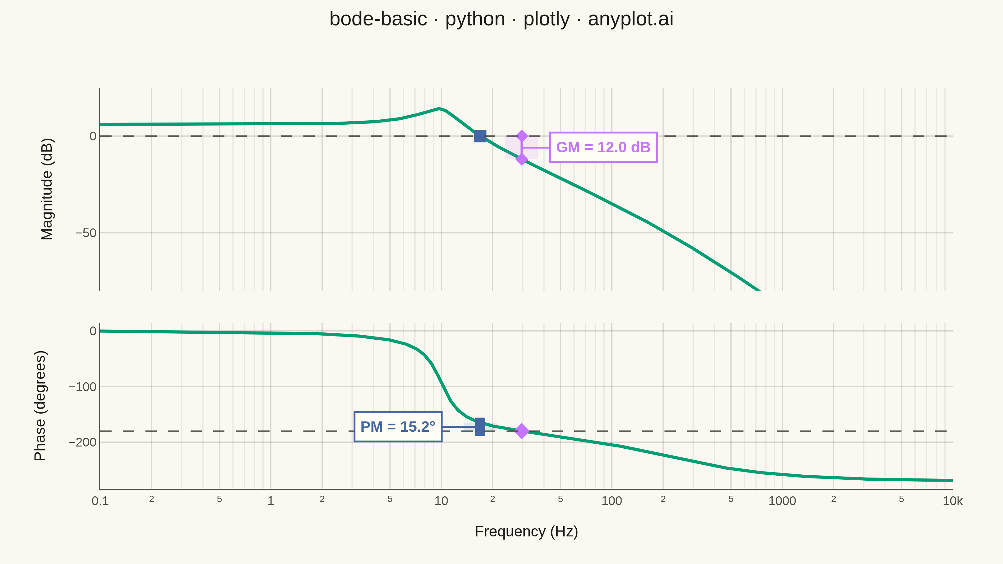
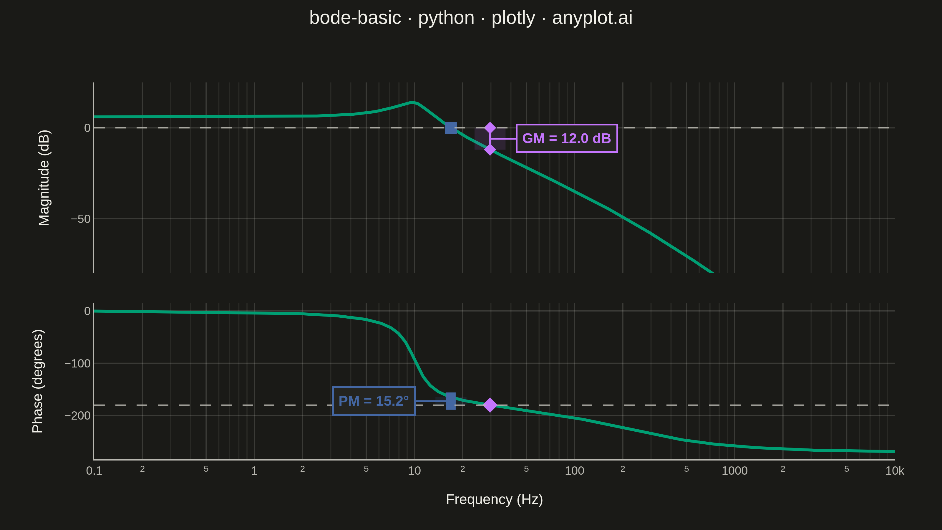
A Bode plot displays a system's frequency response as two vertically aligned panels: magnitude (in decibels) on top and phase (in degrees) on the bottom, both plotted against frequency on a shared logarithmic scale. This visualization is fundamental in control systems engineering and signal processing for analyzing how a system responds to sinusoidal inputs across a range of frequencies, revealing stability characteristics, bandwidth, and resonance behavior.
""" anyplot.ai
bode-basic: Bode Plot for Frequency Response
Library: plotly 6.8.0 | Python 3.13.14
Quality: 93/100 | Updated: 2026-06-17
"""

import os
import sys


# This file is named plotly.py — remove its directory from sys.path so
# 'import plotly' resolves to the installed package, not this script.
_here = os.path.dirname(os.path.abspath(__file__))
sys.path = [p for p in sys.path if os.path.abspath(p or os.getcwd()) != _here]

import numpy as np
import plotly.graph_objects as go
from plotly.subplots import make_subplots


# Theme — Imprint palette chrome tokens
THEME = os.getenv("ANYPLOT_THEME", "light")
PAGE_BG = "#FAF8F1" if THEME == "light" else "#1A1A17"
ELEVATED_BG = "#FFFDF6" if THEME == "light" else "#242420"
INK = "#1A1A17" if THEME == "light" else "#F0EFE8"
INK_SOFT = "#4A4A44" if THEME == "light" else "#B8B7B0"
GRID = "rgba(26,26,23,0.15)" if THEME == "light" else "rgba(240,239,232,0.15)"
GRID_MINOR = "rgba(26,26,23,0.07)" if THEME == "light" else "rgba(240,239,232,0.07)"

# Imprint palette colors — positions 1→3 in canonical order
CLR_MAIN = "#009E73"  # Imprint green (position 1) — main Bode curve
CLR_GAIN = "#C475FD"  # Imprint lavender (position 2) — gain margin annotation
CLR_PHASE = "#4467A3"  # Imprint blue (position 3) — phase margin annotation

# Data — Third-order transfer function: H(s) = K / [(s/p1+1)(s²/wn²+2ζs/wn+1)]
# Complex pair at wn=10 Hz with ζ=0.2 produces a clear resonance peak;
# single real pole at 200 Hz ensures a finite gain margin (phase crosses -180°).
K = 2
p1 = 2 * np.pi * 200  # real pole at 200 Hz (well above resonance)
wn = 2 * np.pi * 10  # resonance at 10 Hz
zeta = 0.2  # underdamped — visible resonance peak

frequency_hz = np.logspace(-1, 4, 800)
omega = 2 * np.pi * frequency_hz
s = 1j * omega

H = K / ((s / p1 + 1) * (s**2 / wn**2 + 2 * zeta * s / wn + 1))
magnitude_db = 20 * np.log10(np.abs(H))
phase_deg = np.degrees(np.unwrap(np.angle(H)))

# Gain crossover: where magnitude crosses 0 dB
gain_cross_idx = np.where(np.diff(np.sign(magnitude_db)))[0]
gc_found = len(gain_cross_idx) > 0
if gc_found:
    gc_idx = gain_cross_idx[-1]
    gc_freq = frequency_hz[gc_idx]
    gc_phase = phase_deg[gc_idx]
    phase_margin = 180 + gc_phase

# Phase crossover: where phase crosses -180 degrees
phase_cross_idx = np.where(np.diff(np.sign(phase_deg + 180)))[0]
pc_found = len(phase_cross_idx) > 0
if pc_found:
    pc_idx = phase_cross_idx[0]
    pc_freq = frequency_hz[pc_idx]
    pc_mag = magnitude_db[pc_idx]
    gain_margin = -pc_mag

# Figure — dual-panel Bode layout
fig = make_subplots(rows=2, cols=1, shared_xaxes=True, vertical_spacing=0.08, row_heights=[0.55, 0.45])

# Magnitude trace (Imprint green — first series)
fig.add_trace(
    go.Scatter(
        x=frequency_hz,
        y=magnitude_db,
        mode="lines",
        line={"color": CLR_MAIN, "width": 2.5},
        name="Magnitude",
        showlegend=False,
    ),
    row=1,
    col=1,
)

# 0 dB reference line (dashed — zeroline suppressed on y-axis to avoid solid overlay)
fig.add_hline(y=0, row=1, col=1, line={"color": INK_SOFT, "width": 1, "dash": "dash"})

# Phase trace (same Imprint green — single-system Bode)
fig.add_trace(
    go.Scatter(
        x=frequency_hz,
        y=phase_deg,
        mode="lines",
        line={"color": CLR_MAIN, "width": 2.5},
        name="Phase",
        showlegend=False,
    ),
    row=2,
    col=1,
)

# -180 degree reference line
fig.add_hline(y=-180, row=2, col=1, line={"color": INK_SOFT, "width": 1, "dash": "dash"})

# Gain margin annotation (Imprint lavender — position 2)
if pc_found:
    fig.add_shape(
        type="rect",
        x0=pc_freq * 0.8,
        x1=pc_freq * 1.25,
        y0=pc_mag,
        y1=0,
        fillcolor=CLR_GAIN,
        opacity=0.12,
        line={"width": 0},
        row=1,
        col=1,
    )
    fig.add_trace(
        go.Scatter(
            x=[pc_freq, pc_freq],
            y=[pc_mag, 0],
            mode="lines+markers",
            line={"color": CLR_GAIN, "width": 2},
            marker={"size": 8, "symbol": "diamond"},
            showlegend=False,
        ),
        row=1,
        col=1,
    )
    fig.add_annotation(
        x=np.log10(pc_freq),
        y=(pc_mag + 0) / 2,
        text=f"<b>GM = {gain_margin:.1f} dB</b>",
        showarrow=True,
        arrowhead=0,
        arrowwidth=1.5,
        arrowcolor=CLR_GAIN,
        ax=65,
        ay=0,
        font={"size": 12, "color": CLR_GAIN},
        bgcolor=ELEVATED_BG,
        bordercolor=CLR_GAIN,
        borderwidth=1.5,
        borderpad=4,
        xref="x",
        yref="y",
        row=1,
        col=1,
    )
    # Cross-panel marker on phase plot
    fig.add_trace(
        go.Scatter(
            x=[pc_freq],
            y=[-180],
            mode="markers",
            marker={"size": 10, "color": CLR_GAIN, "symbol": "diamond"},
            showlegend=False,
        ),
        row=2,
        col=1,
    )

# Phase margin annotation (Imprint blue — position 3)
if gc_found:
    fig.add_shape(
        type="rect",
        x0=gc_freq * 0.8,
        x1=gc_freq * 1.25,
        y0=gc_phase,
        y1=-180,
        fillcolor=CLR_PHASE,
        opacity=0.12,
        line={"width": 0},
        row=2,
        col=1,
    )
    fig.add_trace(
        go.Scatter(
            x=[gc_freq, gc_freq],
            y=[gc_phase, -180],
            mode="lines+markers",
            line={"color": CLR_PHASE, "width": 2, "dash": "dash"},
            marker={"size": 8, "symbol": "square"},
            showlegend=False,
        ),
        row=2,
        col=1,
    )
    fig.add_annotation(
        x=np.log10(gc_freq),
        y=(gc_phase + (-180)) / 2,
        text=f"<b>PM = {phase_margin:.1f}°</b>",
        showarrow=True,
        arrowhead=0,
        arrowwidth=1.5,
        arrowcolor=CLR_PHASE,
        ax=-65,
        ay=0,
        font={"size": 12, "color": CLR_PHASE},
        bgcolor=ELEVATED_BG,
        bordercolor=CLR_PHASE,
        borderwidth=1.5,
        borderpad=4,
        xref="x2",
        yref="y2",
        row=2,
        col=1,
    )
    # Cross-panel marker on magnitude plot
    fig.add_trace(
        go.Scatter(
            x=[gc_freq],
            y=[0],
            mode="markers",
            marker={"size": 10, "color": CLR_PHASE, "symbol": "square"},
            showlegend=False,
        ),
        row=1,
        col=1,
    )

# Layout — theme-adaptive chrome
fig.update_layout(
    autosize=False,
    title={
        "text": "bode-basic · python · plotly · anyplot.ai",
        "font": {"size": 16, "color": INK},
        "x": 0.5,
        "y": 0.98,
    },
    paper_bgcolor=PAGE_BG,
    plot_bgcolor=PAGE_BG,
    font={"color": INK},
    showlegend=False,
    margin={"l": 80, "r": 40, "t": 70, "b": 60},
)

# X-axes (log scale — shared between both panels)
fig.update_xaxes(
    type="log",
    row=2,
    col=1,
    title={"text": "Frequency (Hz)", "font": {"size": 12, "color": INK}},
    tickfont={"size": 10, "color": INK_SOFT},
    showgrid=True,
    gridcolor=GRID,
    gridwidth=1,
    showline=True,
    linecolor=INK_SOFT,
    mirror=False,
    zeroline=False,
    minor={"showgrid": True, "gridcolor": GRID_MINOR},
)
fig.update_xaxes(
    type="log",
    row=1,
    col=1,
    tickfont={"size": 10, "color": INK_SOFT},
    showgrid=True,
    gridcolor=GRID,
    gridwidth=1,
    showline=False,
    linecolor=INK_SOFT,
    mirror=False,
    zeroline=False,
    minor={"showgrid": True, "gridcolor": GRID_MINOR},
)

# Y-axes
fig.update_yaxes(
    row=1,
    col=1,
    title={"text": "Magnitude (dB)", "font": {"size": 12, "color": INK}},
    tickfont={"size": 10, "color": INK_SOFT},
    showgrid=True,
    gridcolor=GRID,
    gridwidth=1,
    showline=True,
    linecolor=INK_SOFT,
    mirror=False,
    zeroline=False,  # suppress solid zeroline so only the dashed add_hline renders
    range=[-80, 25],
)
fig.update_yaxes(
    row=2,
    col=1,
    title={"text": "Phase (degrees)", "font": {"size": 12, "color": INK}},
    tickfont={"size": 10, "color": INK_SOFT},
    showgrid=True,
    gridcolor=GRID,
    gridwidth=1,
    showline=True,
    linecolor=INK_SOFT,
    mirror=False,
    zeroline=False,
)

# Save — landscape 3200 × 1800 (width=800, height=450, scale=4)
fig.write_image(f"plot-{THEME}.png", width=800, height=450, scale=4)
fig.write_html(f"plot-{THEME}.html", include_plotlyjs="cdn")
Runnable source as JSON, for any HTTP client: https://api.anyplot.ai/specs/bode-basic/plotly/code. Any spec id and library id listed in llms-full.txt fit the same URL shape; every URL below is complete and callable.
{
  "spec_id": "bode-basic",
  "language": "python",
  "library": "plotly",
  "page": "https://anyplot.ai/bode-basic/python/plotly",
  "hub": "https://anyplot.ai/bode-basic",
  "code_json": "https://api.anyplot.ai/specs/bode-basic/plotly/code",
  "spec_json": "https://api.anyplot.ai/specs/bode-basic",
  "render_light_png": "https://storage.googleapis.com/anyplot-images/plots/bode-basic/python/plotly/plot-light.png",
  "render_dark_png": "https://storage.googleapis.com/anyplot-images/plots/bode-basic/python/plotly/plot-dark.png",
  "interactive_light_html": "https://storage.googleapis.com/anyplot-images/plots/bode-basic/python/plotly/plot-light.html",
  "interactive_dark_html": "https://storage.googleapis.com/anyplot-images/plots/bode-basic/python/plotly/plot-dark.html",
  "quality_score": 93.0,
  "license": "MIT",
  "guide": "https://anyplot.ai/llms.txt"
}
Part of Bode Plot for Frequency Response on anyplot.ai.