The same plot in 14 other libraries — JavaScript: Chart.js, Apache ECharts, Highcharts, MUI X Charts; Python: Altair, Bokeh, lets-plot, Matplotlib, Plotly, plotnine, Pygal, Seaborn; R: ggplot2; Julia: Makie.jl. Compare all 15 side by side: Calibration Curve in Python, R, Julia and JavaScript.
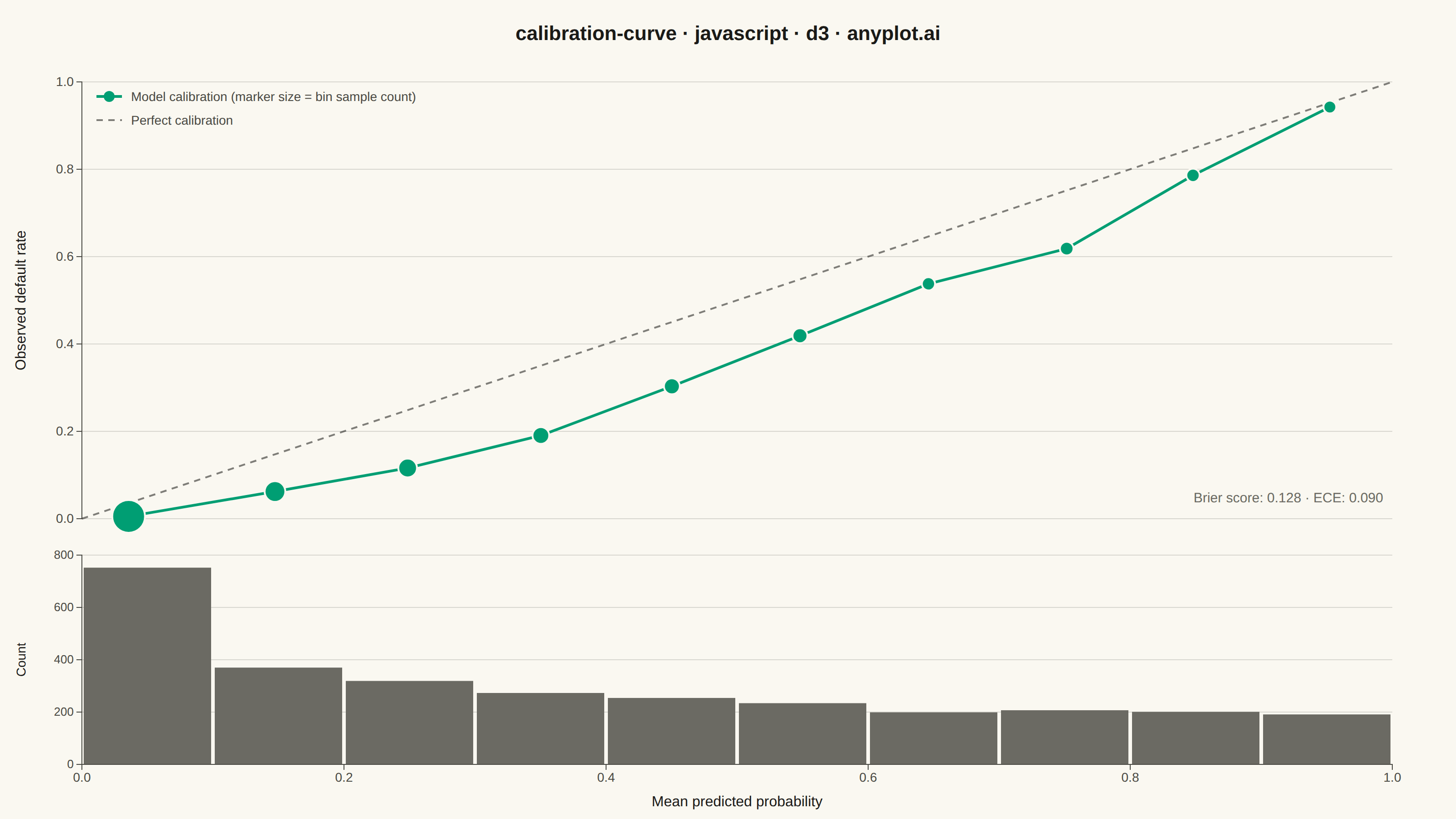
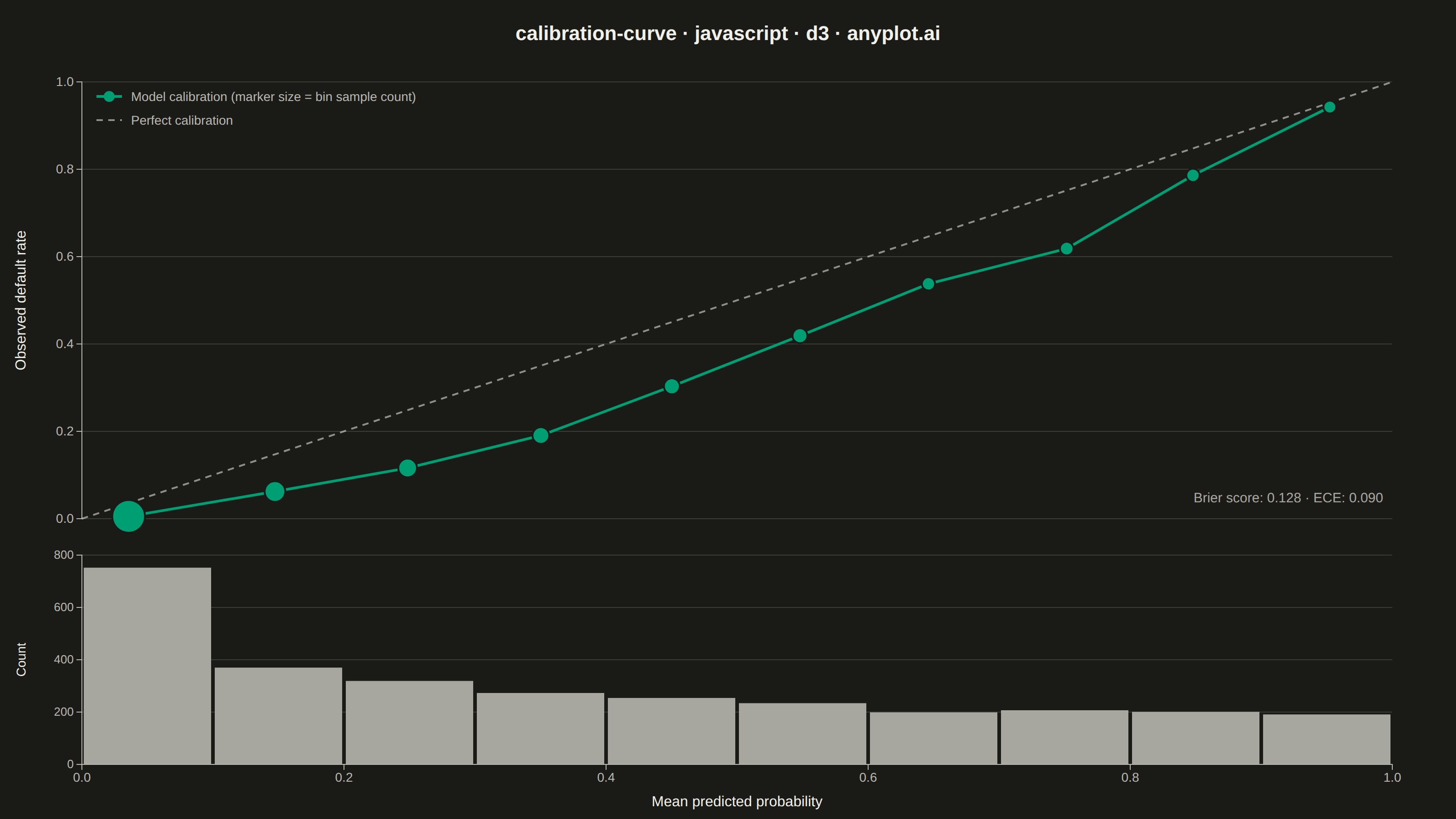
A calibration curve (reliability diagram) visualizes how well the predicted probabilities of a binary classifier match actual outcomes. By plotting the fraction of positives against mean predicted probability in binned intervals, it reveals whether a model is well-calibrated, overconfident, or underconfident. A perfectly calibrated model follows the diagonal line where predicted probability equals observed frequency.
// anyplot.ai
// calibration-curve: Calibration Curve
// Library: d3 7.9.0 | JavaScript 22.23.2
// Quality: 90/100 | Created: 2026-09-02

const t = window.ANYPLOT_TOKENS;
const inkMuted = window.ANYPLOT_THEME === "dark" ? "#A8A79F" : "#6B6A63";
const { width, height } = window.ANYPLOT_SIZE;

// --- Data: a credit-default risk model's predicted probabilities ------------
// Deterministic LCG so the render is reproducible without a network call.
function lcg(seed) {
  let state = seed >>> 0;
  return () => {
    state = (state * 1664525 + 1013904223) >>> 0;
    return state / 4294967296;
  };
}
const rand = lcg(42);

const n = 3000;
const yProb = new Array(n);
const yTrue = new Array(n);
for (let i = 0; i < n; i++) {
  // Most borrowers score low risk; a thin tail scores high risk.
  const predicted = Math.pow(rand(), 1.7);
  // The model is overconfident: true default rates trail the predicted
  // probability, especially in the mid range.
  const truePositiveRate = Math.pow(predicted, 1.5);
  yProb[i] = predicted;
  yTrue[i] = rand() < truePositiveRate ? 1 : 0;
}

const binCount = 10;
const bins = Array.from({ length: binCount }, () => ({ sumProb: 0, sumTrue: 0, count: 0 }));
let sumSquaredError = 0;
for (let i = 0; i < n; i++) {
  const b = bins[Math.min(binCount - 1, Math.floor(yProb[i] * binCount))];
  b.sumProb += yProb[i];
  b.sumTrue += yTrue[i];
  b.count += 1;
  sumSquaredError += (yProb[i] - yTrue[i]) ** 2;
}
const reliability = bins
  .map((b, i) => ({
    binStart: i / binCount,
    binEnd: (i + 1) / binCount,
    meanPred: b.count > 0 ? b.sumProb / b.count : null,
    obsFreq: b.count > 0 ? b.sumTrue / b.count : null,
    count: b.count,
  }))
  .filter((d) => d.count > 0);

const brierScore = sumSquaredError / n;
const ece = reliability.reduce((acc, d) => acc + (d.count / n) * Math.abs(d.obsFreq - d.meanPred), 0);

// --- Layout: reliability plot on top, prediction histogram below ------------
const margin = { top: 90, right: 70, bottom: 60, left: 90 };
const plotWidth = width - margin.left - margin.right;
const calibHeight = 480;
const gap = 40;
const histHeight = height - margin.top - margin.bottom - calibHeight - gap;

const x = d3.scaleLinear().domain([0, 1]).range([0, plotWidth]);
const yCalib = d3.scaleLinear().domain([0, 1]).range([calibHeight, 0]);
const yHist = d3
  .scaleLinear()
  .domain([0, d3.max(reliability, (d) => d.count)])
  .nice()
  .range([histHeight, 0]);
const radius = d3
  .scaleSqrt()
  .domain([d3.min(reliability, (d) => d.count), d3.max(reliability, (d) => d.count)])
  .range([7, 18]);

const svg = d3.select("#container").append("svg").attr("width", width).attr("height", height);

// --- Title --------------------------------------------------------------
svg
  .append("text")
  .attr("x", width / 2)
  .attr("y", 44)
  .attr("text-anchor", "middle")
  .attr("fill", t.ink)
  .style("font-size", "22px")
  .style("font-weight", "600")
  .text("calibration-curve · javascript · d3 · anyplot.ai");

// --- Reliability diagram --------------------------------------------------
const calib = svg.append("g").attr("transform", `translate(${margin.left},${margin.top})`);

calib
  .append("g")
  .attr("class", "grid")
  .call(d3.axisLeft(yCalib).tickValues([0, 0.2, 0.4, 0.6, 0.8, 1]).tickSize(-plotWidth).tickFormat(""))
  .call((g) => g.select(".domain").remove())
  .call((g) => g.selectAll("line").attr("stroke", t.grid));

const calibYAxis = calib.append("g").call(d3.axisLeft(yCalib).tickValues([0, 0.2, 0.4, 0.6, 0.8, 1]).tickFormat(d3.format(".1f")));
calibYAxis.selectAll("text").attr("fill", t.inkSoft).style("font-size", "14px");
calibYAxis.selectAll("line").attr("stroke", t.inkSoft);
calibYAxis.select(".domain").attr("stroke", t.inkSoft);

calib
  .append("text")
  .attr("transform", "rotate(-90)")
  .attr("x", -calibHeight / 2)
  .attr("y", -62)
  .attr("text-anchor", "middle")
  .attr("fill", t.ink)
  .style("font-size", "16px")
  .text("Observed default rate");

// Perfect-calibration reference line — the neutral/baseline semantic anchor.
calib
  .append("line")
  .attr("x1", x(0))
  .attr("y1", yCalib(0))
  .attr("x2", x(1))
  .attr("y2", yCalib(1))
  .attr("stroke", t.ink)
  .attr("stroke-width", 2)
  .attr("stroke-dasharray", "7 6")
  .attr("opacity", 0.55);

const line = d3
  .line()
  .x((d) => x(d.meanPred))
  .y((d) => yCalib(d.obsFreq));

calib
  .append("path")
  .datum(reliability)
  .attr("fill", "none")
  .attr("stroke", t.palette[0])
  .attr("stroke-width", 3)
  .attr("d", line);

calib
  .selectAll("circle")
  .data(reliability)
  .join("circle")
  .attr("cx", (d) => x(d.meanPred))
  .attr("cy", (d) => yCalib(d.obsFreq))
  .attr("r", (d) => radius(d.count))
  .attr("fill", t.palette[0])
  .attr("stroke", t.pageBg)
  .attr("stroke-width", 2);

// Legend
const legend = calib.append("g").attr("transform", "translate(16,16)");
legend.append("line").attr("x1", 0).attr("x2", 28).attr("y1", 0).attr("y2", 0).attr("stroke", t.palette[0]).attr("stroke-width", 3);
legend.append("circle").attr("cx", 14).attr("cy", 0).attr("r", 6).attr("fill", t.palette[0]);
legend
  .append("text")
  .attr("x", 38)
  .attr("y", 5)
  .attr("fill", t.inkSoft)
  .style("font-size", "14px")
  .text("Model calibration (marker size = bin sample count)");
legend
  .append("line")
  .attr("x1", 0)
  .attr("x2", 28)
  .attr("y1", 26)
  .attr("y2", 26)
  .attr("stroke", t.ink)
  .attr("stroke-width", 2)
  .attr("stroke-dasharray", "7 6")
  .attr("opacity", 0.55);
legend.append("text").attr("x", 38).attr("y", 31).attr("fill", t.inkSoft).style("font-size", "14px").text("Perfect calibration");

// Summary metrics — required by the specification. Placed in the empty
// lower-right corner so it never collides with the curve or reference line,
// both of which run through the top-right corner in this scenario.
calib
  .append("text")
  .attr("x", plotWidth - 10)
  .attr("y", calibHeight - 18)
  .attr("text-anchor", "end")
  .attr("fill", inkMuted)
  .style("font-size", "15px")
  .text(`Brier score: ${brierScore.toFixed(3)}  ·  ECE: ${ece.toFixed(3)}`);

// --- Prediction-distribution histogram --------------------------------------
const hist = svg.append("g").attr("transform", `translate(${margin.left},${margin.top + calibHeight + gap})`);

const histYAxis = hist.append("g").call(d3.axisLeft(yHist).ticks(4));
histYAxis.selectAll("text").attr("fill", t.inkSoft).style("font-size", "13px");
histYAxis.selectAll("line").attr("stroke", t.inkSoft);
histYAxis.select(".domain").attr("stroke", t.inkSoft);

hist
  .append("g")
  .attr("class", "grid")
  .call(d3.axisLeft(yHist).ticks(4).tickSize(-plotWidth).tickFormat(""))
  .call((g) => g.select(".domain").remove())
  .call((g) => g.selectAll("line").attr("stroke", t.grid));

hist
  .selectAll("rect")
  .data(reliability)
  .join("rect")
  .attr("x", (d) => x(d.binStart) + 2)
  .attr("width", (d) => Math.max(0, x(d.binEnd) - x(d.binStart) - 4))
  .attr("y", (d) => yHist(d.count))
  .attr("height", (d) => histHeight - yHist(d.count))
  .attr("fill", inkMuted);

const histXAxis = hist.append("g").attr("transform", `translate(0,${histHeight})`).call(d3.axisBottom(x).tickValues([0, 0.2, 0.4, 0.6, 0.8, 1]).tickFormat(d3.format(".1f")));
histXAxis.selectAll("text").attr("fill", t.inkSoft).style("font-size", "14px");
histXAxis.selectAll("line").attr("stroke", t.inkSoft);
histXAxis.select(".domain").attr("stroke", t.inkSoft);

hist
  .append("text")
  .attr("x", plotWidth / 2)
  .attr("y", histHeight + 46)
  .attr("text-anchor", "middle")
  .attr("fill", t.ink)
  .style("font-size", "16px")
  .text("Mean predicted probability");

hist
  .append("text")
  .attr("transform", "rotate(-90)")
  .attr("x", -histHeight / 2)
  .attr("y", -62)
  .attr("text-anchor", "middle")
  .attr("fill", t.ink)
  .style("font-size", "14px")
  .text("Count");
Runnable source as JSON, for any HTTP client: https://api.anyplot.ai/specs/calibration-curve/d3/code. Any spec id and library id listed in llms-full.txt fit the same URL shape; every URL below is complete and callable.
{
  "spec_id": "calibration-curve",
  "language": "javascript",
  "library": "d3",
  "page": "https://anyplot.ai/calibration-curve/javascript/d3",
  "hub": "https://anyplot.ai/calibration-curve",
  "code_json": "https://api.anyplot.ai/specs/calibration-curve/d3/code",
  "spec_json": "https://api.anyplot.ai/specs/calibration-curve",
  "render_light_png": "https://storage.googleapis.com/anyplot-images/plots/calibration-curve/javascript/d3/plot-light.png",
  "render_dark_png": "https://storage.googleapis.com/anyplot-images/plots/calibration-curve/javascript/d3/plot-dark.png",
  "interactive_light_html": "https://storage.googleapis.com/anyplot-images/plots/calibration-curve/javascript/d3/plot-light.html",
  "interactive_dark_html": "https://storage.googleapis.com/anyplot-images/plots/calibration-curve/javascript/d3/plot-dark.html",
  "quality_score": 90.0,
  "license": "MIT",
  "guide": "https://anyplot.ai/llms.txt"
}
Part of Calibration Curve on anyplot.ai.