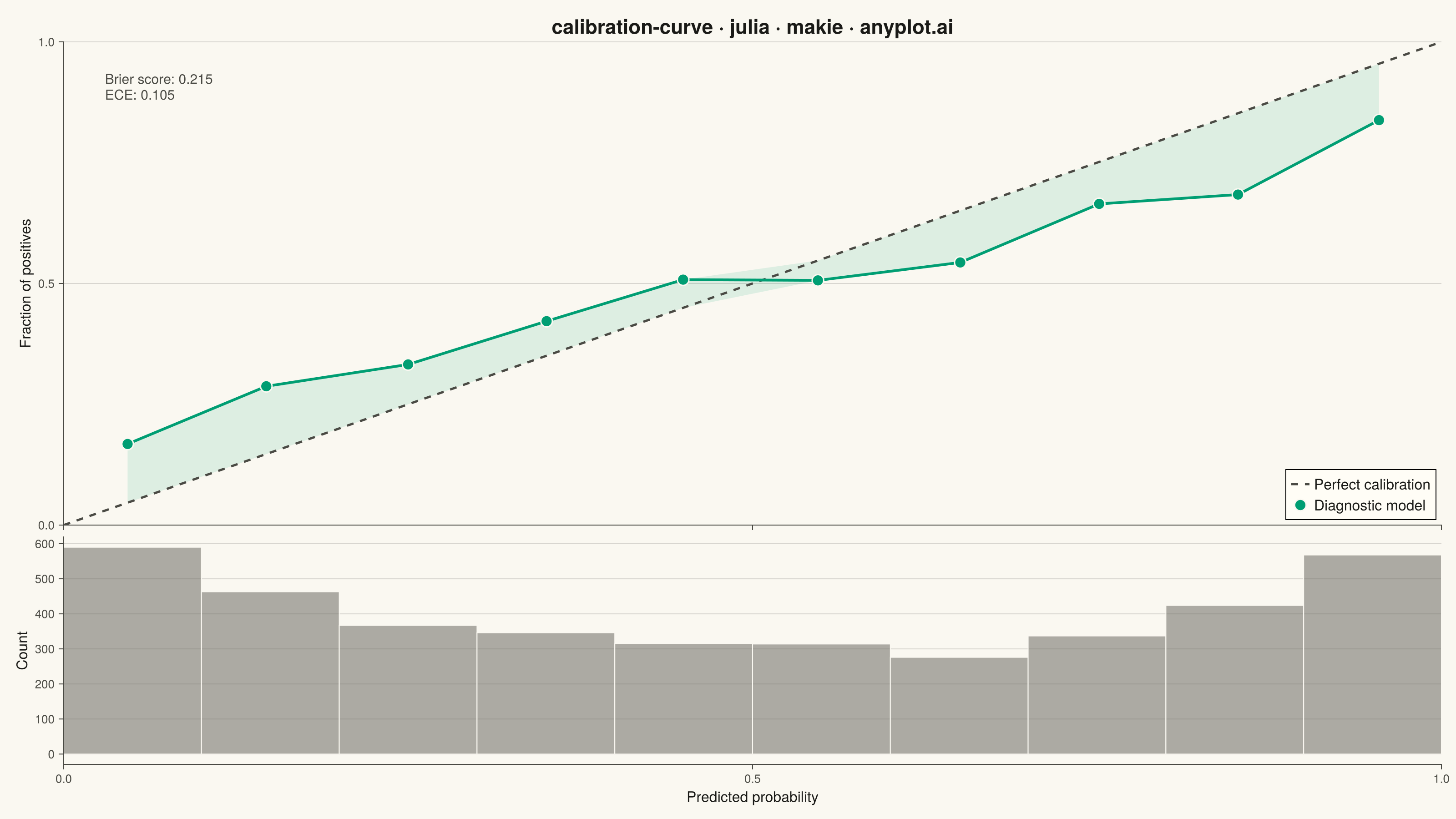
The same plot in 14 other libraries — Python: Altair, Bokeh, lets-plot, Matplotlib, Plotly, plotnine, Pygal, Seaborn; R: ggplot2; JavaScript: Chart.js, D3.js, Apache ECharts, Highcharts, MUI X Charts. Compare all 15 side by side: Calibration Curve in Python, R, Julia and JavaScript.
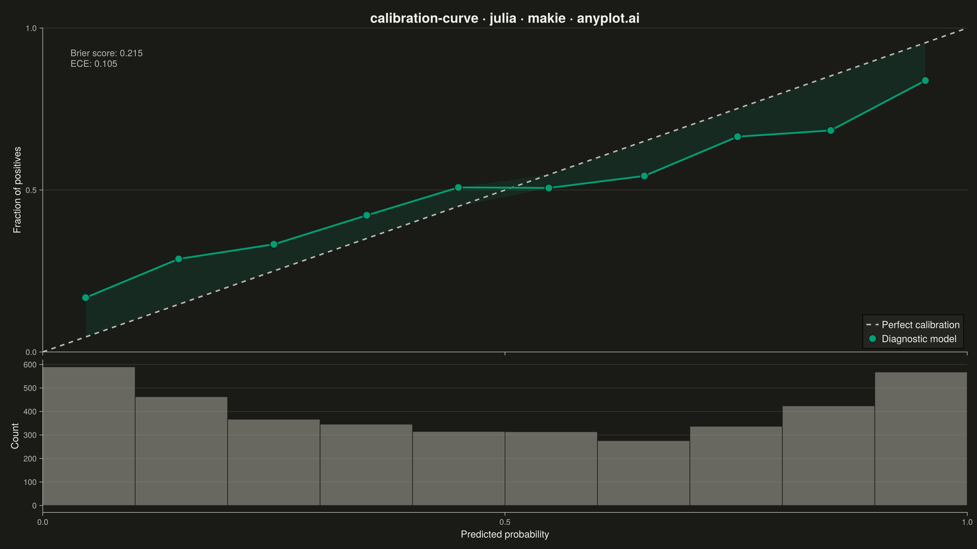
A calibration curve (reliability diagram) visualizes how well the predicted probabilities of a binary classifier match actual outcomes. By plotting the fraction of positives against mean predicted probability in binned intervals, it reveals whether a model is well-calibrated, overconfident, or underconfident. A perfectly calibrated model follows the diagonal line where predicted probability equals observed frequency.
# anyplot.ai
# calibration-curve: Calibration Curve
# Library: makie 0.21.9 | Julia 1.11.9
# Quality: 94/100 | Created: 2026-09-02

using CairoMakie
using Colors
using Random
using Statistics

Random.seed!(42)

# --- Theme tokens -------------------------------------------------------
const THEME      = get(ENV, "ANYPLOT_THEME", "light")
const PAGE_BG    = THEME == "light" ? colorant"#FAF8F1" : colorant"#1A1A17"
const ELEVATED_BG = THEME == "light" ? colorant"#FFFDF6" : colorant"#242420"
const INK        = THEME == "light" ? colorant"#1A1A17" : colorant"#F0EFE8"
const INK_SOFT   = THEME == "light" ? colorant"#4A4A44" : colorant"#B8B7B0"
const INK_MUTED  = THEME == "light" ? colorant"#6B6A63" : colorant"#A8A79F"

const IMPRINT_PALETTE = [
    colorant"#009E73", colorant"#C475FD", colorant"#4467A3", colorant"#BD8233",
    colorant"#AE3030", colorant"#2ABCCD", colorant"#954477", colorant"#99B314",
]
const BRAND = IMPRINT_PALETTE[1]

# --- Data -----------------------------------------------------------------
# Diagnostic screening classifier: a hidden risk score drives the true outcome,
# but the reported probabilities are overconfident (pushed toward 0 and 1).
n = 4000
risk_score = randn(n)
true_prob = 1.0 ./ (1.0 .+ exp.(-1.1 .* risk_score))
y_true = Float64.(rand(n) .< true_prob)

logit_true = log.(true_prob ./ (1.0 .- true_prob))
y_prob = clamp.(1.0 ./ (1.0 .+ exp.(-1.9 .* logit_true .+ 0.15 .* randn(n))), 0.001, 0.999)

n_bins = 10
edges = range(0.0, 1.0; length = n_bins + 1)
mean_pred = fill(NaN, n_bins)
frac_pos = fill(NaN, n_bins)
bin_count = zeros(Int, n_bins)

for i in 1:n_bins
    lo, hi = edges[i], edges[i + 1]
    mask = i < n_bins ? (y_prob .>= lo) .& (y_prob .< hi) : (y_prob .>= lo) .& (y_prob .<= hi)
    bin_count[i] = count(mask)
    if bin_count[i] > 0
        mean_pred[i] = mean(y_prob[mask])
        frac_pos[i] = mean(y_true[mask])
    end
end

valid = bin_count .> 0
mp = mean_pred[valid]
fp = frac_pos[valid]
brier_score = mean((y_prob .- y_true) .^ 2)
ece = sum(bin_count[valid] ./ n .* abs.(fp .- mp))

# --- Plot -------------------------------------------------------------------
fig = Figure(
    size            = (1600, 900),
    fontsize        = 16,
    backgroundcolor = PAGE_BG,
)

ax_cal = Axis(
    fig[1, 1];
    title             = "calibration-curve · julia · makie · anyplot.ai",
    titlesize         = 22,
    titlecolor        = INK,
    ylabel            = "Fraction of positives",
    ylabelcolor       = INK,
    ylabelsize        = 16,
    xticklabelsize    = 13,
    yticklabelsize    = 13,
    xticklabelcolor   = INK_SOFT,
    yticklabelcolor   = INK_SOFT,
    xtickcolor        = INK_SOFT,
    ytickcolor        = INK_SOFT,
    backgroundcolor   = PAGE_BG,
    topspinevisible   = false,
    rightspinevisible = false,
    leftspinecolor    = INK_SOFT,
    bottomspinecolor  = INK_SOFT,
    xgridvisible      = false,
    ygridcolor        = RGBAf(INK.r, INK.g, INK.b, 0.15),
    xminorgridvisible = false,
    yminorgridvisible = false,
    limits            = (0, 1, 0, 1),
)

band!(ax_cal, mp, min.(fp, mp), max.(fp, mp); color = (BRAND, 0.12))
lines!(ax_cal, [0.0, 1.0], [0.0, 1.0];
    color = INK_SOFT, linestyle = :dash, linewidth = 2.5, label = "Perfect calibration")
lines!(ax_cal, mp, fp; color = BRAND, linewidth = 3)
scatter!(ax_cal, mp, fp; color = BRAND, markersize = 18, strokewidth = 1.5, strokecolor = PAGE_BG, label = "Diagnostic model")

axislegend(ax_cal, position = :rb, framevisible = true, backgroundcolor = ELEVATED_BG, labelcolor = INK)

text!(ax_cal, 0.03, 0.94;
    text = "Brier score: $(round(brier_score, digits = 3))\nECE: $(round(ece, digits = 3))",
    color = INK_SOFT, fontsize = 15, align = (:left, :top))

hidexdecorations!(ax_cal; label = true, ticklabels = true, ticks = false, grid = false)

ax_hist = Axis(
    fig[2, 1];
    xlabel            = "Predicted probability",
    ylabel            = "Count",
    xlabelcolor       = INK,
    ylabelcolor       = INK,
    xlabelsize        = 16,
    ylabelsize        = 16,
    xticklabelsize    = 13,
    yticklabelsize    = 13,
    xticklabelcolor   = INK_SOFT,
    yticklabelcolor   = INK_SOFT,
    xtickcolor        = INK_SOFT,
    ytickcolor        = INK_SOFT,
    backgroundcolor   = PAGE_BG,
    topspinevisible   = false,
    rightspinevisible = false,
    leftspinecolor    = INK_SOFT,
    bottomspinecolor  = INK_SOFT,
    xgridvisible      = false,
    ygridcolor        = RGBAf(INK.r, INK.g, INK.b, 0.15),
    limits            = (0, 1, nothing, nothing),
)

hist!(ax_hist, y_prob; bins = edges, color = (INK_MUTED, 0.55), strokewidth = 1, strokecolor = PAGE_BG)

linkxaxes!(ax_cal, ax_hist)
rowsize!(fig.layout, 1, Relative(0.68))
rowsize!(fig.layout, 2, Relative(0.32))
rowgap!(fig.layout, 8)

# --- Save -------------------------------------------------------------------
save("plot-$(THEME).png", fig; px_per_unit = 2)
Runnable source as JSON, for any HTTP client: https://api.anyplot.ai/specs/calibration-curve/makie/code. Any spec id and library id listed in llms-full.txt fit the same URL shape; every URL below is complete and callable.
{
  "spec_id": "calibration-curve",
  "language": "julia",
  "library": "makie",
  "page": "https://anyplot.ai/calibration-curve/julia/makie",
  "hub": "https://anyplot.ai/calibration-curve",
  "code_json": "https://api.anyplot.ai/specs/calibration-curve/makie/code",
  "spec_json": "https://api.anyplot.ai/specs/calibration-curve",
  "render_light_png": "https://storage.googleapis.com/anyplot-images/plots/calibration-curve/julia/makie/plot-light.png",
  "render_dark_png": "https://storage.googleapis.com/anyplot-images/plots/calibration-curve/julia/makie/plot-dark.png",
  "quality_score": 94.0,
  "license": "MIT",
  "guide": "https://anyplot.ai/llms.txt"
}
Part of Calibration Curve on anyplot.ai.