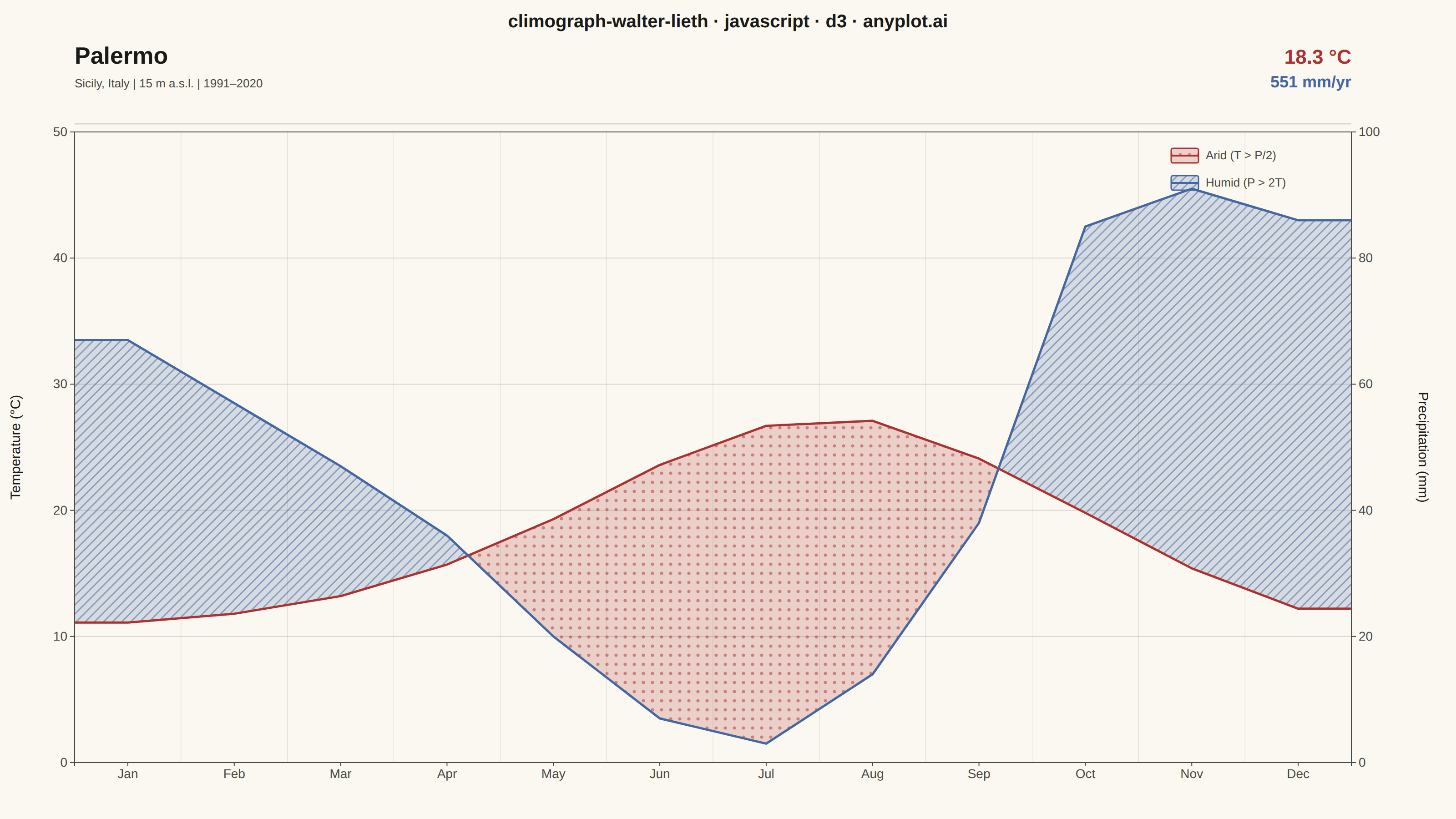
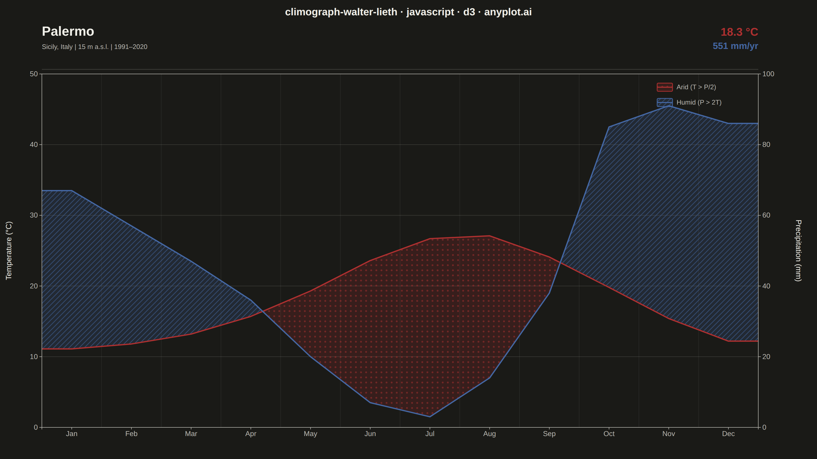
A Walter-Lieth climate diagram (climograph) is the canonical visualization of a location's annual climate, plotting monthly mean temperature and monthly precipitation over the twelve months on a single panel. It uses the classic 1:2 axis-scaling convention where 10 °C on the temperature axis aligns with 20 mm on the precipitation axis, so the relationship between the two curves directly reveals water availability: where precipitation exceeds the temperature curve the period is humid (filled blue/hatched), and where the temperature curve rises above precipitation the period is arid (filled red/dotted). A header carries station metadata and annual means, while frost indicators along the baseline mark cold months.
// anyplot.ai
// climograph-walter-lieth: Walter-Lieth Climate Diagram
// Library: d3 7.9.0 | JavaScript 22.22.3
// Quality: 93/100 | Created: 2026-06-15

const t = window.ANYPLOT_TOKENS;
const { width, height } = window.ANYPLOT_SIZE;

// Palermo, Sicily — classic Mediterranean climate, 1991–2020 normals
const station = {
  name: "Palermo",
  region: "Sicily, Italy",
  elevation: 15,
  tempMean: 18.3,
  precipTotal: 551,
  period: "1991–2020",
};
const MONTHS  = ["Jan","Feb","Mar","Apr","May","Jun","Jul","Aug","Sep","Oct","Nov","Dec"];
const temps   = [11.1, 11.8, 13.2, 15.7, 19.3, 23.6, 26.7, 27.1, 24.1, 19.8, 15.4, 12.2];
const precips = [  67,   57,   47,   36,   20,    7,    3,   14,   38,   85,   91,   86];
const data    = MONTHS.map((month, i) => ({ month, temp: temps[i], precip: precips[i] }));

// Walter-Lieth convention: 10 °C ↔ 20 mm (2:1 ratio)
// Bottom = 0 °C / 0 mm; top = 50 °C / 100 mm (perhumid threshold)
const TEMP_MIN = 0;
const TEMP_MAX = 50;

const margin = { top: 145, right: 115, bottom: 62, left: 82 };
const iw = width  - margin.left - margin.right;
const ih = height - margin.top  - margin.bottom;

// Semantic colors: temperature → Imprint red, precipitation → Imprint blue
const TEMP_COLOR = "#AE3030";
const PRCP_COLOR = "#4467A3";

// ── SVG root ────────────────────────────────────────────────────────────────
const svg = d3.select("#container").append("svg")
  .attr("width", width).attr("height", height);

const g = svg.append("g").attr("transform", `translate(${margin.left},${margin.top})`);

// ── Scales ──────────────────────────────────────────────────────────────────
const xScale  = d3.scaleBand().domain(MONTHS).range([0, iw]).padding(0);
const yTemp   = d3.scaleLinear().domain([TEMP_MIN, TEMP_MAX]).range([ih, 0]);
// Right-axis scale mirrors temperature scale at 2:1 ratio (0–100 mm = 0–50 °C)
const yPrcpAx = d3.scaleLinear().domain([0, 100]).range([ih, 0]);

// Precipitation → pixel (2:1 ratio; above 100 mm compressed to 10:1)
const yP = (mm) => mm <= 100 ? yTemp(mm / 2) : yTemp(50 + (mm - 100) * 0.1);

// x center of each month band
const xMid = (d) => xScale(d.month) + xScale.bandwidth() / 2;

// Coordinate arrays in group-local space
const tPts = data.map((d) => [xMid(d), yTemp(d.temp)]);
const pPts = data.map((d) => [xMid(d), yP(d.precip)]);

// ── SVG <defs>: fill patterns + masks ──────────────────────────────────────
const defs = svg.append("defs");

// Arid fill pattern — red dots on translucent red ground (Walter-Lieth "dotted")
const aPat = defs.append("pattern").attr("id", "aridPat")
  .attr("patternUnits", "userSpaceOnUse").attr("width", 10).attr("height", 10);
aPat.append("rect").attr("width", 10).attr("height", 10).attr("fill", "rgba(174,48,48,0.20)");
aPat.append("circle").attr("cx", 5).attr("cy", 5).attr("r", 1.8)
  .attr("fill", "rgba(174,48,48,0.50)");

// Humid fill pattern — diagonal hatching on translucent blue ground (Walter-Lieth "hatched")
const hPat = defs.append("pattern").attr("id", "humidPat")
  .attr("patternUnits", "userSpaceOnUse").attr("width", 10).attr("height", 10);
hPat.append("rect").attr("width", 10).attr("height", 10).attr("fill", "rgba(68,103,163,0.20)");
[[-5, 5, 5, -5],[0, 10, 10, 0],[5, 15, 15, 5]].forEach(([x1, y1, x2, y2]) => {
  hPat.append("line").attr("x1", x1).attr("y1", y1).attr("x2", x2).attr("y2", y2)
    .attr("stroke", "rgba(68,103,163,0.55)").attr("stroke-width", 1.5);
});

// Closed polygon "below the curve", extended to the full plot width
// Mask coordinates are in group-local space (0→iw, 0→ih)
const belowPath = (pts) => {
  let d = `M0,${ih} L0,${pts[0][1]}`;
  pts.forEach(([x, y]) => { d += ` L${x},${y}`; });
  d += ` L${iw},${pts[pts.length - 1][1]} L${iw},${ih} Z`;
  return d;
};

// SVG mask: show (below primaryPts) minus (below subtractPts)
const addMask = (id, primaryPts, subtractPts) => {
  const m = defs.append("mask").attr("id", id);
  m.append("rect").attr("x", 0).attr("y", 0).attr("width", iw).attr("height", ih)
    .attr("fill", "black");
  m.append("path").attr("d", belowPath(primaryPts)).attr("fill", "white");
  m.append("path").attr("d", belowPath(subtractPts)).attr("fill", "black");
};

addMask("aridMask",  tPts, pPts); // below temp curve AND above precip curve → arid
addMask("humidMask", pPts, tPts); // below precip curve AND above temp curve → humid

// ── Grid lines ───────────────────────────────────────────────────────────────
g.append("g").selectAll("line").data([0, 10, 20, 30, 40, 50]).join("line")
  .attr("x1", 0).attr("x2", iw)
  .attr("y1", (v) => yTemp(v)).attr("y2", (v) => yTemp(v))
  .attr("stroke", t.grid).attr("stroke-width", 1);

// Vertical month dividers (subtle)
MONTHS.forEach((m) => {
  g.append("line")
    .attr("x1", xScale(m)).attr("x2", xScale(m))
    .attr("y1", 0).attr("y2", ih)
    .attr("stroke", t.grid).attr("stroke-width", 0.5);
});

// ── Filled areas (pattern + mask) ────────────────────────────────────────────
g.append("rect").attr("width", iw).attr("height", ih)
  .attr("fill", "url(#aridPat)").attr("mask", "url(#aridMask)");
g.append("rect").attr("width", iw).attr("height", ih)
  .attr("fill", "url(#humidPat)").attr("mask", "url(#humidMask)");

// ── Data lines ───────────────────────────────────────────────────────────────
// Lines extended to full plot width for a clean edge-to-edge look
const extLinePath = (pts) => {
  const ex = [[0, pts[0][1]], ...pts, [iw, pts[pts.length - 1][1]]];
  return "M" + ex.map(([x, y]) => `${x},${y}`).join(" L");
};

g.append("path").attr("d", extLinePath(tPts))
  .attr("fill", "none").attr("stroke", TEMP_COLOR)
  .attr("stroke-width", 2.5).attr("stroke-linejoin", "round");

g.append("path").attr("d", extLinePath(pPts))
  .attr("fill", "none").attr("stroke", PRCP_COLOR)
  .attr("stroke-width", 2.5).attr("stroke-linejoin", "round");

// ── Left axis: Temperature (°C) ──────────────────────────────────────────────
const axL = g.append("g").call(
  d3.axisLeft(yTemp).tickValues([0, 10, 20, 30, 40, 50])
    .tickSize(5).tickFormat(d3.format("d"))
);
axL.selectAll("text").attr("fill", t.inkSoft).style("font-size", "14px");
axL.selectAll(".tick line").attr("stroke", t.inkSoft);
axL.select(".domain").attr("stroke", t.inkSoft);

g.append("text")
  .attr("transform", `translate(-60,${ih / 2}) rotate(-90)`)
  .attr("text-anchor", "middle").attr("fill", t.ink).style("font-size", "15px")
  .text("Temperature (°C)");

// ── Right axis: Precipitation (mm) ───────────────────────────────────────────
const axR = g.append("g").attr("transform", `translate(${iw},0)`).call(
  d3.axisRight(yPrcpAx).tickValues([0, 20, 40, 60, 80, 100])
    .tickSize(5).tickFormat(d3.format("d"))
);
axR.selectAll("text").attr("fill", t.inkSoft).style("font-size", "14px");
axR.selectAll(".tick line").attr("stroke", t.inkSoft);
axR.select(".domain").attr("stroke", t.inkSoft);

g.append("text")
  .attr("transform", `translate(${iw + 74},${ih / 2}) rotate(90)`)
  .attr("text-anchor", "middle").attr("fill", t.ink).style("font-size", "15px")
  .text("Precipitation (mm)");

// ── Bottom axis: Months ───────────────────────────────────────────────────────
const axB = g.append("g").attr("transform", `translate(0,${ih})`).call(
  d3.axisBottom(xScale).tickSize(4)
);
axB.selectAll("text").attr("fill", t.inkSoft).style("font-size", "14px");
axB.selectAll(".tick line").attr("stroke", t.inkSoft);
axB.select(".domain").attr("stroke", t.inkSoft);

// ── Header ────────────────────────────────────────────────────────────────────
// Mandated anyplot title
svg.append("text").attr("x", width / 2).attr("y", 30)
  .attr("text-anchor", "middle").attr("fill", t.ink)
  .style("font-size", "20px").style("font-weight", "600")
  .text("climograph-walter-lieth · javascript · d3 · anyplot.ai");

// Station name
svg.append("text").attr("x", margin.left).attr("y", 70)
  .attr("fill", t.ink).style("font-size", "26px").style("font-weight", "700")
  .text(station.name);

// Location and period
svg.append("text").attr("x", margin.left).attr("y", 96)
  .attr("fill", t.inkSoft).style("font-size", "13px")
  .text(`${station.region}  |  ${station.elevation} m a.s.l.  |  ${station.period}`);

// Annual mean temperature (right side of header)
const hx = width - margin.right;
svg.append("text").attr("x", hx).attr("y", 70).attr("text-anchor", "end")
  .attr("fill", TEMP_COLOR).style("font-size", "22px").style("font-weight", "700")
  .text(`${station.tempMean} °C`);

svg.append("text").attr("x", hx).attr("y", 96).attr("text-anchor", "end")
  .attr("fill", PRCP_COLOR).style("font-size", "18px").style("font-weight", "600")
  .text(`${station.precipTotal} mm/yr`);

// Separator line below header
svg.append("line")
  .attr("x1", margin.left).attr("x2", width - margin.right)
  .attr("y1", margin.top - 9).attr("y2", margin.top - 9)
  .attr("stroke", t.grid).attr("stroke-width", 1.5);

// ── Plot border ───────────────────────────────────────────────────────────────
g.append("rect").attr("width", iw).attr("height", ih)
  .attr("fill", "none").attr("stroke", t.inkSoft).attr("stroke-width", 1);

// ── Legend ────────────────────────────────────────────────────────────────────
const lx = iw - 198, ly = 18;
const legItems = [
  { patId: "aridPat",  lineColor: TEMP_COLOR, label: "Arid  (T > P/2)" },
  { patId: "humidPat", lineColor: PRCP_COLOR, label: "Humid  (P > 2T)" },
];
legItems.forEach(({ patId, lineColor, label }, i) => {
  const y0 = ly + i * 30;
  g.append("rect").attr("x", lx).attr("y", y0).attr("width", 30).attr("height", 16)
    .attr("fill", `url(#${patId})`).attr("stroke", lineColor).attr("stroke-width", 1.5)
    .attr("rx", 2);
  g.append("line").attr("x1", lx).attr("x2", lx + 30)
    .attr("y1", y0 + 8).attr("y2", y0 + 8)
    .attr("stroke", lineColor).attr("stroke-width", 2);
  g.append("text").attr("x", lx + 38).attr("y", y0 + 12)
    .attr("fill", t.inkSoft).style("font-size", "13px").text(label);
});
Runnable source as JSON, for any HTTP client: https://api.anyplot.ai/specs/climograph-walter-lieth/d3/code. Any spec id and library id listed in llms-full.txt fit the same URL shape; every URL below is complete and callable.
{
  "spec_id": "climograph-walter-lieth",
  "language": "javascript",
  "library": "d3",
  "page": "https://anyplot.ai/climograph-walter-lieth/javascript/d3",
  "hub": "https://anyplot.ai/climograph-walter-lieth",
  "code_json": "https://api.anyplot.ai/specs/climograph-walter-lieth/d3/code",
  "spec_json": "https://api.anyplot.ai/specs/climograph-walter-lieth",
  "render_light_png": "https://storage.googleapis.com/anyplot-images/plots/climograph-walter-lieth/javascript/d3/plot-light.png",
  "render_dark_png": "https://storage.googleapis.com/anyplot-images/plots/climograph-walter-lieth/javascript/d3/plot-dark.png",
  "interactive_light_html": "https://storage.googleapis.com/anyplot-images/plots/climograph-walter-lieth/javascript/d3/plot-light.html",
  "interactive_dark_html": "https://storage.googleapis.com/anyplot-images/plots/climograph-walter-lieth/javascript/d3/plot-dark.html",
  "quality_score": 93.0,
  "license": "MIT",
  "guide": "https://anyplot.ai/llms.txt"
}
Part of Walter-Lieth Climate Diagram on anyplot.ai.