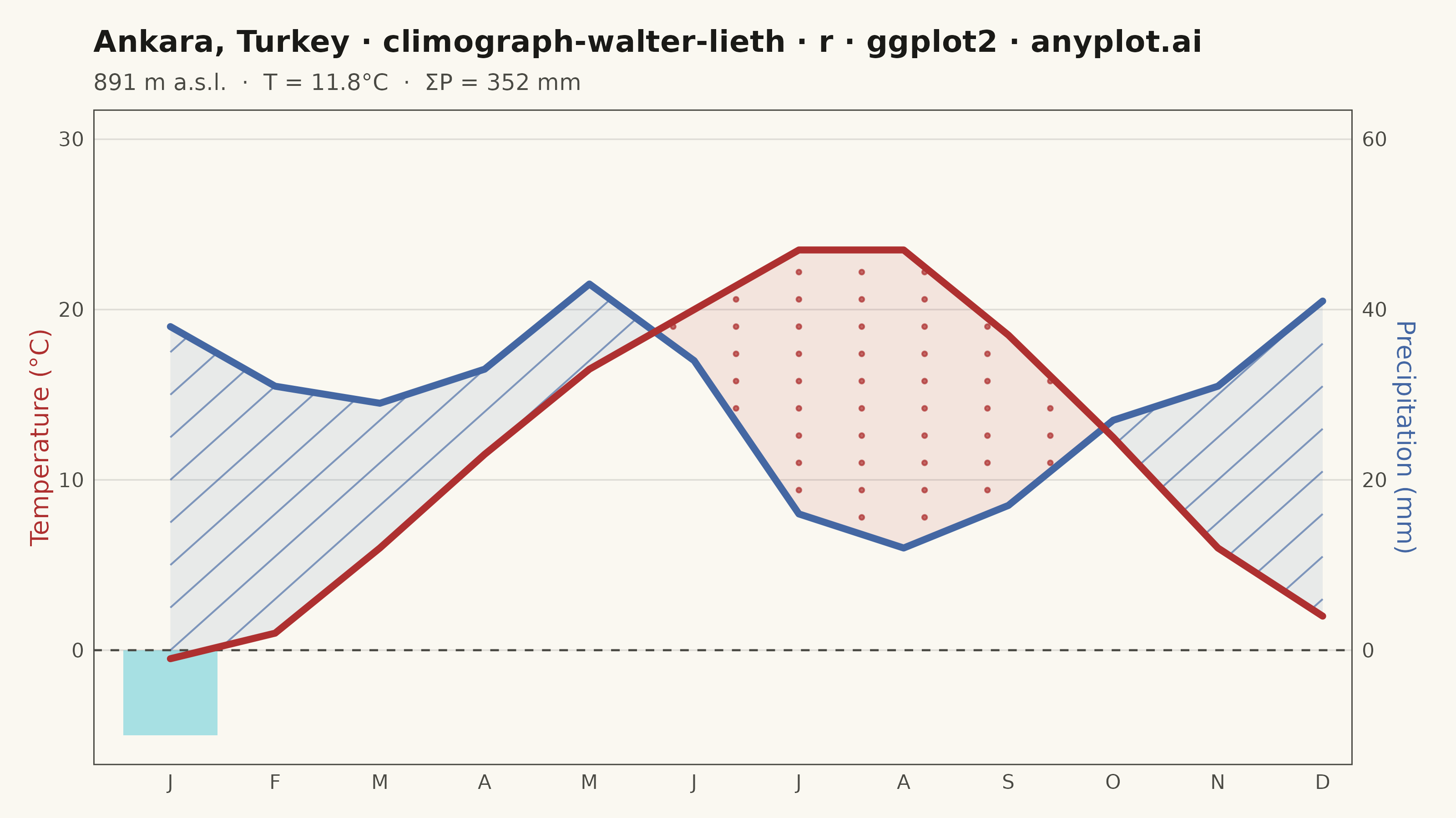
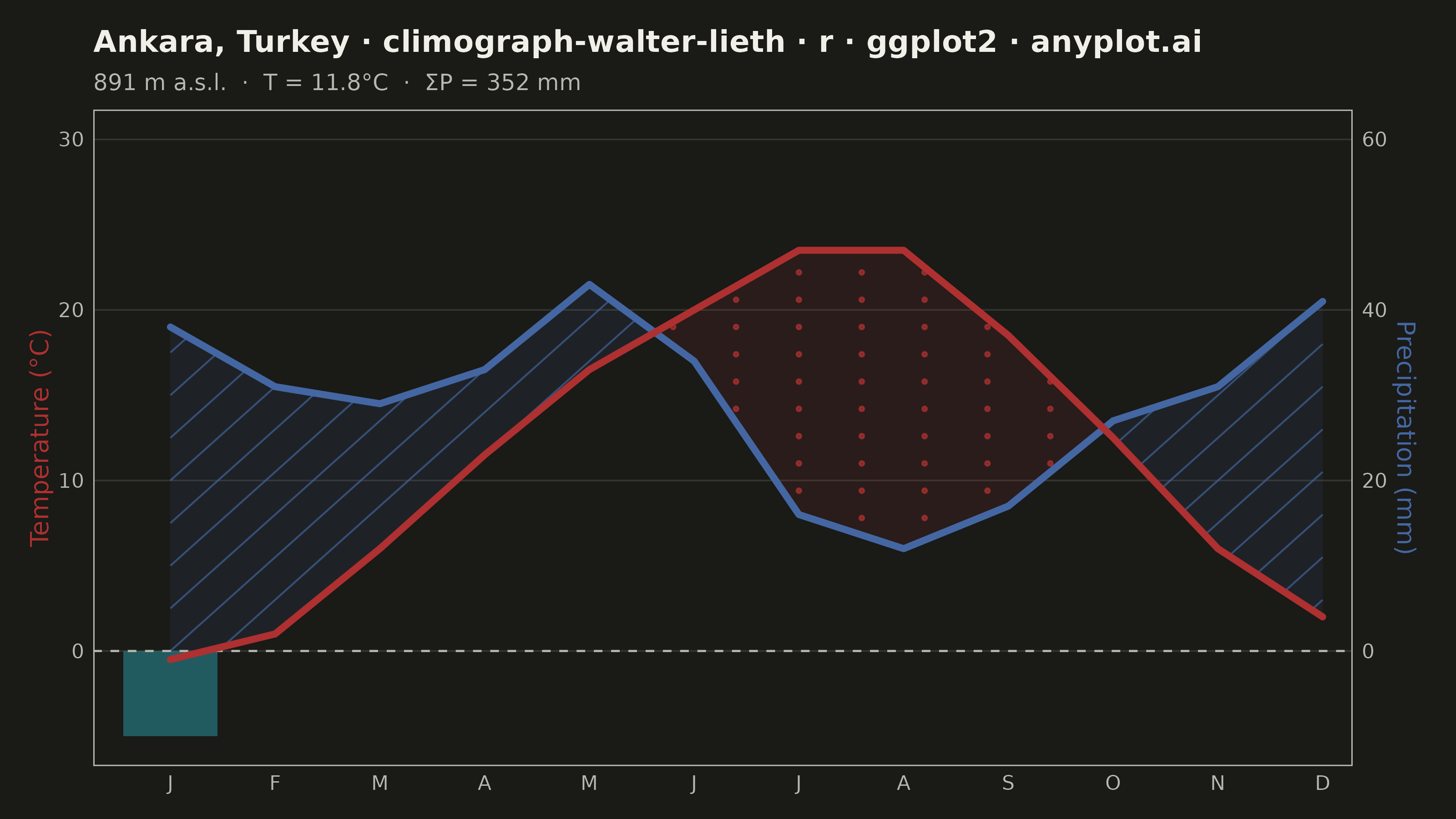
A Walter-Lieth climate diagram (climograph) is the canonical visualization of a location's annual climate, plotting monthly mean temperature and monthly precipitation over the twelve months on a single panel. It uses the classic 1:2 axis-scaling convention where 10 °C on the temperature axis aligns with 20 mm on the precipitation axis, so the relationship between the two curves directly reveals water availability: where precipitation exceeds the temperature curve the period is humid (filled blue/hatched), and where the temperature curve rises above precipitation the period is arid (filled red/dotted). A header carries station metadata and annual means, while frost indicators along the baseline mark cold months.
#' anyplot.ai
#' climograph-walter-lieth: Walter-Lieth Climate Diagram
#' Library: ggplot2 3.5.1 | R 4.4.1
#' Quality: 92/100 | Created: 2026-06-15

library(ggplot2)
library(ragg)

# Theme tokens (Imprint palette — theme-adaptive chrome)
THEME       <- Sys.getenv("ANYPLOT_THEME", "light")
PAGE_BG     <- if (THEME == "light") "#FAF8F1" else "#1A1A17"
ELEVATED_BG <- if (THEME == "light") "#FFFDF6" else "#242420"
INK         <- if (THEME == "light") "#1A1A17" else "#F0EFE8"
INK_SOFT    <- if (THEME == "light") "#4A4A44" else "#B8B7B0"
INK_MUTED   <- if (THEME == "light") "#6B6A63" else "#A8A79F"

# Imprint categorical palette (hybrid-v3 sort order)
IMPRINT_PALETTE <- c(
  "#009E73",  # 1 — brand green (first categorical series)
  "#C475FD",  # 2 — lavender
  "#4467A3",  # 3 — blue
  "#BD8233",  # 4 — ochre
  "#AE3030",  # 5 — matte red
  "#2ABCCD",  # 6 — cyan
  "#954477",  # 7 — rose
  "#99B314"   # 8 — lime
)

# Domain-convention colors (semantic exception: temperature→red, precipitation→blue/water)
COLOR_TEMP   <- IMPRINT_PALETTE[5]           # #AE3030 — temperature (hot/warm semantic)
COLOR_PRECIP <- IMPRINT_PALETTE[3]           # #4467A3 — precipitation (water semantic)
COLOR_FROST  <- IMPRINT_PALETTE[6]           # #2ABCCD — frost period (cold/ice semantic)
GRID_COLOR   <- adjustcolor(INK, alpha.f = 0.12)

# Station metadata — Ankara, Turkey (continental climate with summer arid period)
station_elev        <- 891
annual_mean_temp    <- 11.8
annual_precip_total <- 352

# Monthly climate normals (1991-2020 reference period)
climate_df <- data.frame(
  month_idx = 1:12,
  month_lbl = c("J", "F", "M", "A", "M", "J", "J", "A", "S", "O", "N", "D"),
  temp      = c(-0.5,  1.0,  6.0, 11.5, 16.5, 20.0, 23.5, 23.5, 18.5, 12.5,  6.0,  2.0),
  precip    = c( 38.0, 31.0, 29.0, 33.0, 43.0, 34.0, 16.0, 12.0, 17.0, 27.0, 31.0, 41.0)
)

# Walter-Lieth 1:2 scaling convention: 10°C aligns with 20 mm on the shared axis
climate_df$prec_scaled <- climate_df$precip / 2

# Smooth interpolation between months for continuous fill regions
n_interp <- 600
x_smooth <- seq(1, 12, length.out = n_interp)
t_smooth <- approx(climate_df$month_idx, climate_df$temp,        x_smooth)$y
p_smooth <- approx(climate_df$month_idx, climate_df$prec_scaled, x_smooth)$y
p_smooth <- pmin(p_smooth, 50)  # cap at 100 mm / 2 = 50 (standard WL scale maximum)

# Ribbon endpoints for thin background tint under pattern fills
fill_df <- data.frame(
  x          = x_smooth,
  temp       = t_smooth,
  prec_s     = p_smooth,
  humid_ymax = pmax(t_smooth, p_smooth),
  arid_ymin  = pmin(t_smooth, p_smooth)
)

# --- Diagonal hatching for humid region (precipitation > temperature curve) ---
# Slope chosen so hatch lines appear at ~45 degrees on 8×4.5-inch canvas
# (x range 11 units at 8/11 in/unit, y range 35 units at ~4.1/35 in/unit → slope ≈ 5.5)
hatch_slope     <- 5.5   # dy/dx in data coordinates
hatch_spacing_y <- 2.5   # y-intercept spacing between parallel lines

# Intercepts: must cover y ∈ [-0.5, 21] at x ∈ [1,12]; at x=12: y = 60.5 + b
hatch_intercepts <- seq(-65, 25, by = hatch_spacing_y)

hatch_seg_list <- lapply(hatch_intercepts, function(b) {
  y_line  <- hatch_slope * (x_smooth - 1) + b
  in_humid <- p_smooth > t_smooth & y_line >= t_smooth & y_line <= p_smooth
  if (!any(in_humid)) return(NULL)
  rle_res <- rle(in_humid)
  pos <- 1L
  k   <- 0L
  out_list <- vector("list", sum(rle_res$values))
  for (i in seq_along(rle_res$lengths)) {
    len <- rle_res$lengths[i]
    if (rle_res$values[i]) {
      k <- k + 1L
      end_pos <- pos + len - 1L
      out_list[[k]] <- data.frame(
        x    = x_smooth[pos],    xend = x_smooth[end_pos],
        y    = y_line[pos],      yend = y_line[end_pos]
      )
    }
    pos <- pos + len
  }
  if (k > 0L) do.call(rbind, out_list[seq_len(k)]) else NULL
})
hatch_seg_df <- do.call(rbind, Filter(Negate(is.null), hatch_seg_list))

# --- Stipple dots for arid region (temperature > precipitation curve) ---
x_dot_seq <- seq(1, 12, by = 0.6)
y_dot_seq <- seq(-5, 30, by = 1.6)
dot_grid  <- expand.grid(x = x_dot_seq, y = y_dot_seq)
dot_grid$t_at_x <- approx(x_smooth, t_smooth, dot_grid$x, rule = 2)$y
dot_grid$p_at_x <- approx(x_smooth, p_smooth, dot_grid$x, rule = 2)$y
arid_dots <- dot_grid[
  dot_grid$t_at_x > dot_grid$p_at_x &
  dot_grid$y      >= dot_grid$p_at_x &
  dot_grid$y      <= dot_grid$t_at_x, ]

# Frost-month rectangles (mean temperature below 0°C)
frost_months <- climate_df$month_idx[climate_df$temp < 0]
frost_df <- if (length(frost_months) > 0) {
  data.frame(
    xmin = frost_months - 0.45,
    xmax = frost_months + 0.45
  )
} else {
  NULL
}

# Plot title — mandatory anyplot format with descriptive station prefix
plot_title <- paste0(
  "Ankara, Turkey · climograph-walter-lieth · r · ggplot2 · anyplot.ai"
)
title_fontsize <- max(8L, round(12L * min(1.0, 67 / nchar(plot_title))))

# Subtitle carries the station header (Walter-Lieth convention)
plot_subtitle <- sprintf(
  "%d m a.s.l.  ·  T = %.1f°C  ·  ΣP = %d mm",
  station_elev, annual_mean_temp, as.integer(annual_precip_total)
)

# Build plot
p <- ggplot() +
  # Humid background tint (blue, very light) under the hatching
  geom_ribbon(
    data = fill_df,
    aes(x = x, ymin = temp, ymax = humid_ymax),
    fill = COLOR_PRECIP, alpha = 0.10, inherit.aes = FALSE
  ) +
  # Diagonal hatching lines for humid period (blue/hatched per Walter-Lieth convention)
  (if (!is.null(hatch_seg_df) && nrow(hatch_seg_df) > 0)
    geom_segment(
      data = hatch_seg_df,
      aes(x = x, xend = xend, y = y, yend = yend),
      color = COLOR_PRECIP, linewidth = 0.35, alpha = 0.65, inherit.aes = FALSE
    )
  else NULL) +
  # Arid background tint (red, very light) under the stipple dots
  geom_ribbon(
    data = fill_df,
    aes(x = x, ymin = arid_ymin, ymax = temp),
    fill = COLOR_TEMP, alpha = 0.10, inherit.aes = FALSE
  ) +
  # Stipple dots for arid period (red/dotted per Walter-Lieth convention)
  (if (nrow(arid_dots) > 0)
    geom_point(
      data = arid_dots,
      aes(x = x, y = y),
      color = COLOR_TEMP, size = 0.55, alpha = 0.70, inherit.aes = FALSE
    )
  else NULL) +
  # Frost-month indicator bands below 0°C
  (if (!is.null(frost_df))
    geom_rect(
      data = frost_df,
      aes(xmin = xmin, xmax = xmax),
      ymin = -5, ymax = 0,
      fill = COLOR_FROST, alpha = 0.40, inherit.aes = FALSE
    )
  else NULL) +
  # Frost threshold reference line
  geom_hline(yintercept = 0, color = INK_SOFT, linewidth = 0.4, linetype = "dashed") +
  # Precipitation curve (plotted at precip/2 on temp axis; right axis shows actual mm)
  geom_line(
    data = climate_df,
    aes(x = month_idx, y = prec_scaled),
    color = COLOR_PRECIP, linewidth = 1.3, lineend = "round"
  ) +
  # Temperature curve
  geom_line(
    data = climate_df,
    aes(x = month_idx, y = temp),
    color = COLOR_TEMP, linewidth = 1.3, lineend = "round"
  ) +
  # X axis: month abbreviations
  scale_x_continuous(
    breaks = 1:12,
    labels = c("J", "F", "M", "A", "M", "J", "J", "A", "S", "O", "N", "D"),
    expand = c(0.025, 0)
  ) +
  # Dual y-axis: left = temperature (°C), right = precipitation (mm) at 2× scale
  scale_y_continuous(
    name   = "Temperature (°C)",
    limits = c(-5, 30),
    breaks = c(0, 10, 20, 30),
    sec.axis = sec_axis(
      ~ . * 2,
      name   = "Precipitation (mm)",
      breaks = c(0, 20, 40, 60),
      labels = c("0", "20", "40", "60")
    )
  ) +
  labs(
    title    = plot_title,
    subtitle = plot_subtitle,
    x        = NULL
  ) +
  theme_minimal(base_size = 8) +
  theme(
    plot.background    = element_rect(fill = PAGE_BG, color = PAGE_BG),
    panel.background   = element_rect(fill = PAGE_BG, color = NA),
    panel.grid.major.y = element_line(color = GRID_COLOR, linewidth = 0.3),
    panel.grid.major.x = element_blank(),
    panel.grid.minor   = element_blank(),
    panel.border       = element_rect(color = INK_SOFT, fill = NA, linewidth = 0.5),
    axis.title.y.left  = element_text(color = COLOR_TEMP,   size = 10),
    axis.title.y.right = element_text(color = COLOR_PRECIP, size = 10),
    axis.text.y.left   = element_text(color = INK_SOFT, size = 8),
    axis.text.y.right  = element_text(color = INK_SOFT, size = 8),
    axis.text.x        = element_text(color = INK_SOFT, size = 8),
    axis.line          = element_blank(),
    plot.title         = element_text(color = INK, size = title_fontsize, face = "bold"),
    plot.subtitle      = element_text(color = INK_SOFT, size = 9,
                                      margin = margin(t = 2, b = 6)),
    plot.margin        = margin(12, 16, 10, 12, "pt")
  )

# Save (landscape: 8 × 4.5 in @ 400 dpi → 3200 × 1800 px)
ggsave(
  filename = sprintf("plot-%s.png", THEME),
  plot     = p,
  device   = ragg::agg_png,
  width    = 8,
  height   = 4.5,
  units    = "in",
  dpi      = 400
)
Runnable source as JSON, for any HTTP client: https://api.anyplot.ai/specs/climograph-walter-lieth/ggplot2/code. Any spec id and library id listed in llms-full.txt fit the same URL shape; every URL below is complete and callable.
{
  "spec_id": "climograph-walter-lieth",
  "language": "r",
  "library": "ggplot2",
  "page": "https://anyplot.ai/climograph-walter-lieth/r/ggplot2",
  "hub": "https://anyplot.ai/climograph-walter-lieth",
  "code_json": "https://api.anyplot.ai/specs/climograph-walter-lieth/ggplot2/code",
  "spec_json": "https://api.anyplot.ai/specs/climograph-walter-lieth",
  "render_light_png": "https://storage.googleapis.com/anyplot-images/plots/climograph-walter-lieth/r/ggplot2/plot-light.png",
  "render_dark_png": "https://storage.googleapis.com/anyplot-images/plots/climograph-walter-lieth/r/ggplot2/plot-dark.png",
  "quality_score": 92.0,
  "license": "MIT",
  "guide": "https://anyplot.ai/llms.txt"
}
Part of Walter-Lieth Climate Diagram on anyplot.ai.