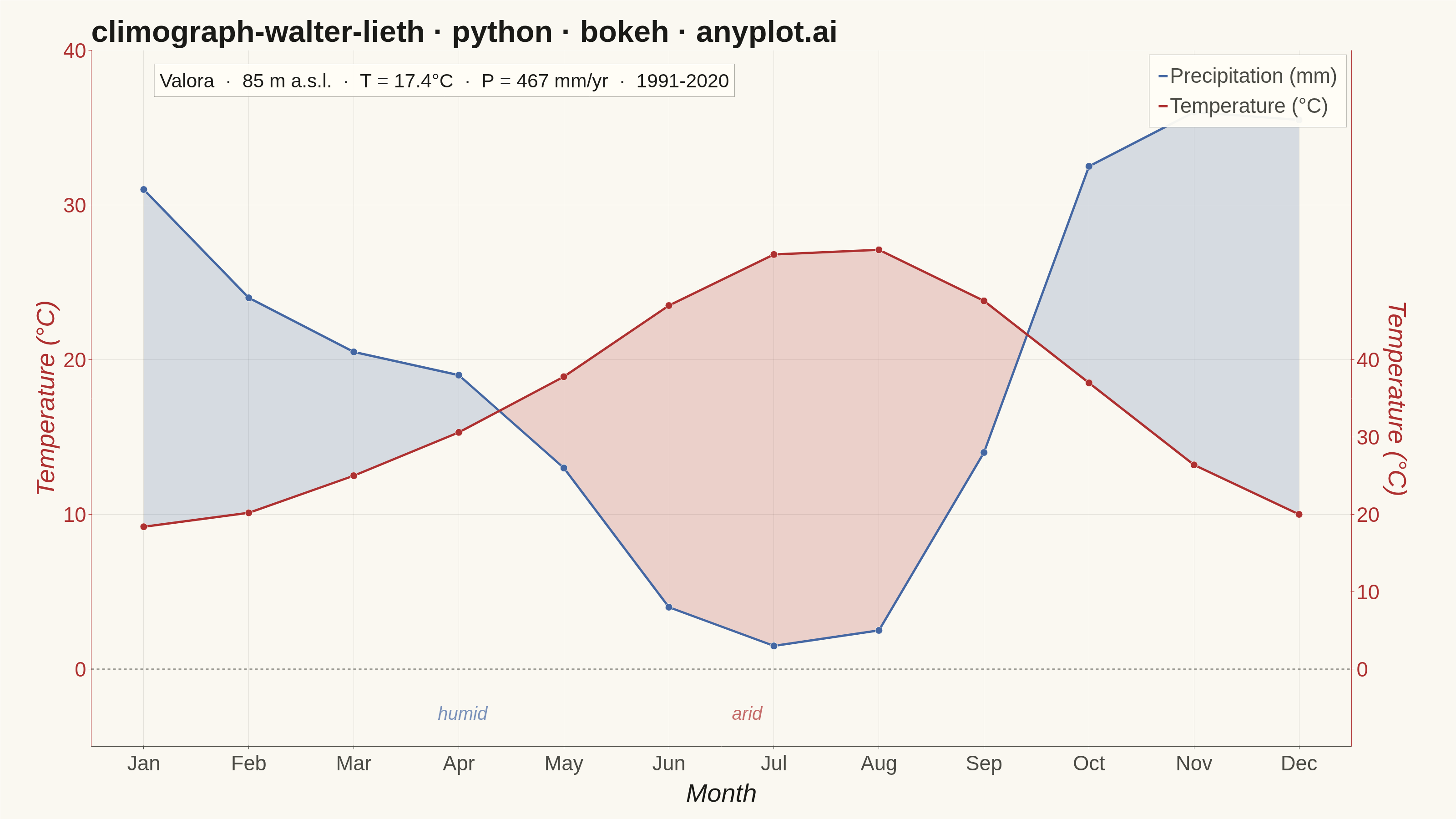
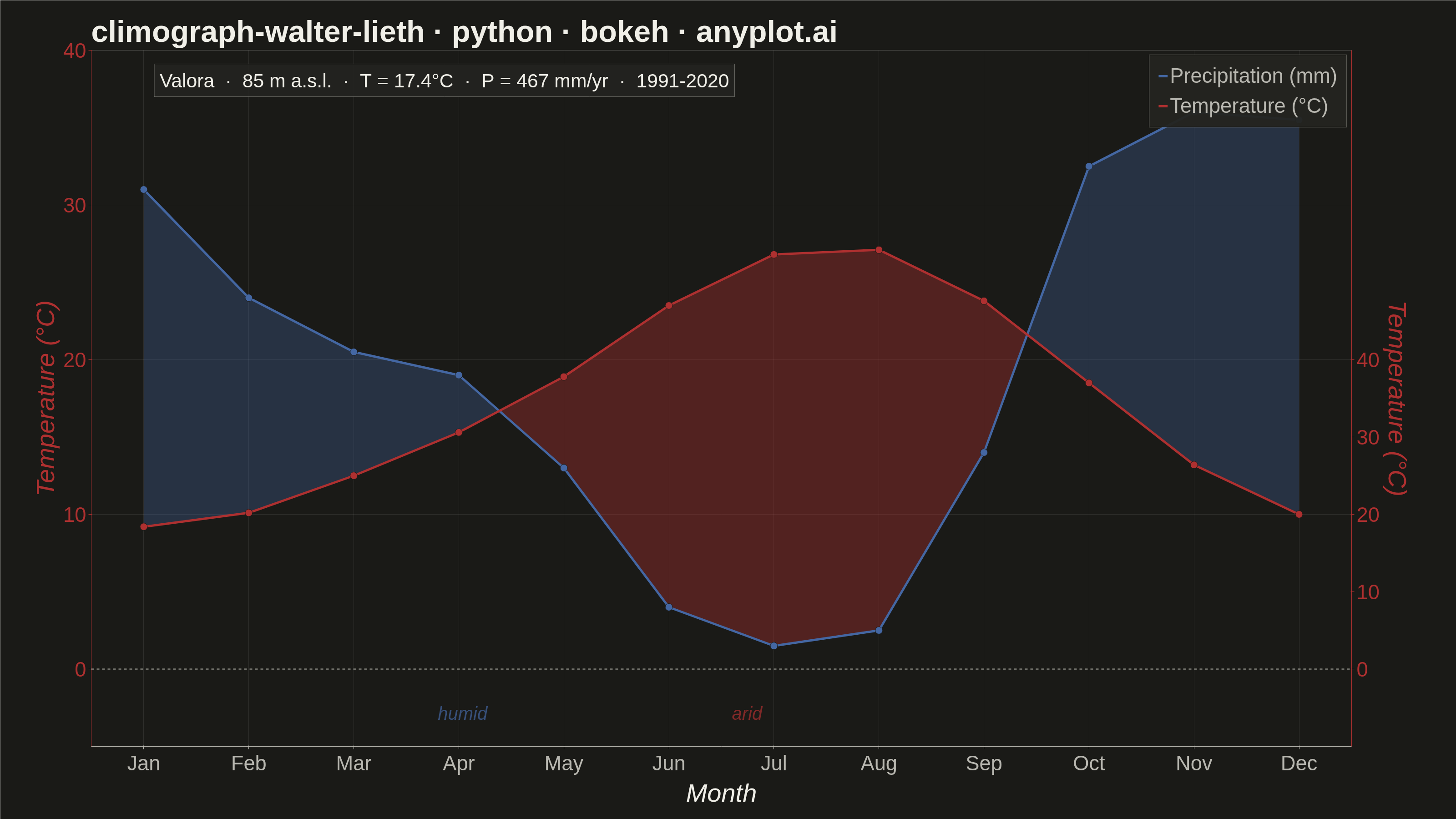
A Walter-Lieth climate diagram (climograph) is the canonical visualization of a location's annual climate, plotting monthly mean temperature and monthly precipitation over the twelve months on a single panel. It uses the classic 1:2 axis-scaling convention where 10 °C on the temperature axis aligns with 20 mm on the precipitation axis, so the relationship between the two curves directly reveals water availability: where precipitation exceeds the temperature curve the period is humid (filled blue/hatched), and where the temperature curve rises above precipitation the period is arid (filled red/dotted). A header carries station metadata and annual means, while frost indicators along the baseline mark cold months.
""" anyplot.ai
climograph-walter-lieth: Walter-Lieth Climate Diagram
Library: bokeh 3.9.1 | Python 3.13.13
Quality: 91/100 | Created: 2026-06-15
"""

import io
import os
import sys
import time
from pathlib import Path


# Remove current dir from sys.path so bokeh.py doesn't shadow the bokeh package
sys.path = [p for p in sys.path if p != "" and not (os.path.isfile(os.path.join(p, "bokeh.py")) if p else False)]

import numpy as np
from bokeh.io import output_file, save
from bokeh.models import CustomJSTickFormatter, FixedTicker, Label, LinearAxis, Range1d, Span
from bokeh.plotting import figure
from PIL import Image
from selenium import webdriver
from selenium.webdriver.chrome.options import Options


# Theme tokens
THEME = os.getenv("ANYPLOT_THEME", "light")
PAGE_BG = "#FAF8F1" if THEME == "light" else "#1A1A17"
ELEVATED_BG = "#FFFDF6" if THEME == "light" else "#242420"
INK = "#1A1A17" if THEME == "light" else "#F0EFE8"
INK_SOFT = "#4A4A44" if THEME == "light" else "#B8B7B0"
INK_MUTED = "#6B6A63" if THEME == "light" else "#A8A79F"

# Imprint palette — semantic assignments for Walter-Lieth
TEMP_COLOR = "#AE3030"  # matte red (heat / temperature)
PRECIP_COLOR = "#4467A3"  # blue (water / precipitation)

# Data — Mediterranean coastal station "Valora" (fictional), 1991-2020 normals
STATION_NAME = "Valora"
ELEVATION_M = 85
temperature = np.array([9.2, 10.1, 12.5, 15.3, 18.9, 23.5, 26.8, 27.1, 23.8, 18.5, 13.2, 10.0])
precipitation = np.array([62.0, 48.0, 41.0, 38.0, 26.0, 8.0, 3.0, 5.0, 28.0, 65.0, 72.0, 71.0])

annual_mean_temp = temperature.mean()
annual_total_precip = precipitation.sum()

# Walter-Lieth scaling: 10 deg-C <-> 20 mm  =>  temp-scale precip = precip / 2
x_idx = np.arange(12, dtype=float)
temp_equiv = precipitation / 2.0  # precipitation mapped to left (temp) axis

# Fine interpolation for smooth fill polygons at curve crossings
x_fine = np.linspace(0, 11, 1200)
temp_fine = np.interp(x_fine, x_idx, temperature)
tequiv_fine = np.interp(x_fine, x_idx, temp_equiv)

# Humid fill: where temp_equiv > temp (precipitation curve above temperature line)
humid_mask = tequiv_fine > temp_fine
y1_humid = np.where(humid_mask, tequiv_fine, temp_fine)
y2_humid = temp_fine

# Arid fill: where temp > temp_equiv (temperature line above precipitation curve)
arid_mask = temp_fine > tequiv_fine
y1_arid = np.where(arid_mask, temp_fine, tequiv_fine)
y2_arid = tequiv_fine

# Axis ranges — left (temperature) and right (precipitation = 2x temperature)
T_MIN, T_MAX = -5.0, 40.0
P_MIN, P_MAX = T_MIN * 2, T_MAX * 2  # -10, 80 mm

# Title length scaling
title_str = "climograph-walter-lieth · python · bokeh · anyplot.ai"
n = len(title_str)
ratio = 67 / n if n > 67 else 1.0
title_size = f"{max(34, round(50 * ratio))}pt"

# Build figure
p = figure(
    width=3200,
    height=1800,
    x_range=Range1d(-0.5, 11.5),
    y_range=Range1d(T_MIN, T_MAX),
    toolbar_location=None,
    min_border_bottom=160,
    min_border_left=200,
    min_border_top=110,
    min_border_right=230,
)

# Theme
p.background_fill_color = PAGE_BG
p.border_fill_color = PAGE_BG
p.outline_line_color = None

# Precipitation right axis (range 2x the temperature range for 1:2 Walter-Lieth scaling)
p.extra_y_ranges = {"precip": Range1d(P_MIN, P_MAX)}
right_ax = LinearAxis(
    y_range_name="precip",
    axis_label="Precipitation (mm)",
    ticker=FixedTicker(ticks=[0, 20, 40, 60, 80]),
    axis_label_text_font_size="42pt",
    axis_label_text_color=PRECIP_COLOR,
    major_label_text_font_size="34pt",
    major_label_text_color=PRECIP_COLOR,
    axis_line_color=PRECIP_COLOR,
    major_tick_line_color=PRECIP_COLOR,
    minor_tick_line_color=PRECIP_COLOR,
)
p.add_layout(right_ax, "right")

# Humid fill (blue — precipitation curve above temperature line)
# Higher alpha in dark theme to compensate for low contrast on near-black background
HUMID_ALPHA = 0.32 if THEME == "dark" else 0.20
ARID_ALPHA = 0.38 if THEME == "dark" else 0.20
p.varea(x=x_fine, y1=y1_humid, y2=y2_humid, fill_color=PRECIP_COLOR, fill_alpha=HUMID_ALPHA)

# Arid fill (red — temperature line above precipitation curve)
p.varea(x=x_fine, y1=y1_arid, y2=y2_arid, fill_color=TEMP_COLOR, fill_alpha=ARID_ALPHA)

# Precipitation line (plotted in temperature-scale units on left axis)
p.line(x=x_idx, y=temp_equiv, line_color=PRECIP_COLOR, line_width=5, legend_label="Precipitation (mm)")

# Temperature line
p.line(x=x_idx, y=temperature, line_color=TEMP_COLOR, line_width=5, legend_label="Temperature (°C)")

# Dots on lines for month markers
p.scatter(x=x_idx, y=temperature, fill_color=TEMP_COLOR, line_color=PAGE_BG, size=16)
p.scatter(x=x_idx, y=temp_equiv, fill_color=PRECIP_COLOR, line_color=PAGE_BG, size=16)

# Zero-degree reference line
p.add_layout(Span(location=0, dimension="width", line_color=INK_SOFT, line_width=2, line_dash="dashed"))

# Frost indicator — blue blocks below x-axis for months with mean temp < 0
for i, t in enumerate(temperature):
    if t < 0:
        p.varea(x=[i - 0.45, i + 0.45], y1=[T_MIN, T_MIN], y2=[0.0, 0.0], fill_color=PRECIP_COLOR, fill_alpha=0.45)

# Title
p.title.text = title_str
p.title.text_font_size = title_size
p.title.text_color = INK
p.title.text_font_style = "bold"

# Station metadata annotation — placed inside the plot at the top center
# (the area above y≈28°C in summer months is free of data in a Mediterranean chart)
station_header = (
    f"{STATION_NAME}  ·  {ELEVATION_M} m a.s.l.  ·  "
    f"T = {annual_mean_temp:.1f}°C  ·  "
    f"P = {annual_total_precip:.0f} mm/yr  ·  1991-2020"
)
p.add_layout(
    Label(
        x=0.1,
        y=37.0,
        text=station_header,
        text_font_size="32pt",
        text_color=INK,
        background_fill_color=ELEVATED_BG,
        background_fill_alpha=0.90,
        border_line_color=INK_SOFT,
        border_line_alpha=0.50,
        padding=12,
    )
)

# Left axis (temperature — colored red to match line)
p.yaxis.axis_label = "Temperature (°C)"
p.yaxis.axis_label_text_font_size = "42pt"
p.yaxis.axis_label_text_color = TEMP_COLOR
p.yaxis.major_label_text_font_size = "34pt"
p.yaxis.major_label_text_color = TEMP_COLOR
p.yaxis.axis_line_color = TEMP_COLOR
p.yaxis.major_tick_line_color = TEMP_COLOR
p.yaxis.minor_tick_line_color = TEMP_COLOR
p.yaxis.ticker = FixedTicker(ticks=[0, 10, 20, 30, 40])

# X-axis (months)
p.xaxis.axis_label = "Month"
p.xaxis.axis_label_text_font_size = "42pt"
p.xaxis.axis_label_text_color = INK
p.xaxis.major_label_text_font_size = "34pt"
p.xaxis.major_label_text_color = INK_SOFT
p.xaxis.axis_line_color = INK_SOFT
p.xaxis.major_tick_line_color = INK_SOFT
p.xaxis.minor_tick_line_color = INK_SOFT
p.xaxis.ticker = FixedTicker(ticks=list(range(12)))
p.xaxis.formatter = CustomJSTickFormatter(
    code="""
    const labels = ['Jan','Feb','Mar','Apr','May','Jun',
                    'Jul','Aug','Sep','Oct','Nov','Dec'];
    return (tick >= 0 && tick <= 11) ? labels[tick] : '';
"""
)

# Grid
p.xgrid.grid_line_color = INK
p.xgrid.grid_line_alpha = 0.10
p.xgrid.grid_line_width = 1
p.ygrid.grid_line_color = INK
p.ygrid.grid_line_alpha = 0.10
p.ygrid.grid_line_width = 1

# Legend
p.legend.location = "top_right"
p.legend.background_fill_color = ELEVATED_BG
p.legend.border_line_color = INK_SOFT
p.legend.label_text_color = INK_SOFT
p.legend.label_text_font_size = "34pt"
p.legend.padding = 20
p.legend.spacing = 14

# Humid/arid period labels inside plot (bottom center)
p.add_layout(
    Label(
        x=2.8,
        y=T_MIN + 1.5,
        text="humid",
        text_font_size="30pt",
        text_color=PRECIP_COLOR,
        text_alpha=0.70,
        text_font_style="italic",
    )
)
p.add_layout(
    Label(
        x=5.6,
        y=T_MIN + 1.5,
        text="arid",
        text_font_size="30pt",
        text_color=TEMP_COLOR,
        text_alpha=0.70,
        text_font_style="italic",
    )
)

# Save interactive HTML
output_file(f"plot-{THEME}.html")
save(p)

# Screenshot via Selenium — window taller than target so browser overhead
# does not clip the figure; PIL crops to the exact 3200x1800 canvas.
FIG_W, FIG_H = 3200, 1800
WIN_W, WIN_H = FIG_W, FIG_H + 200
opts = Options()
for arg in (
    "--headless=new",
    "--no-sandbox",
    "--disable-dev-shm-usage",
    "--disable-gpu",
    f"--window-size={WIN_W},{WIN_H}",
    "--hide-scrollbars",
):
    opts.add_argument(arg)
driver = webdriver.Chrome(options=opts)
driver.set_window_size(WIN_W, WIN_H)
driver.get(f"file://{Path(f'plot-{THEME}.html').resolve()}")
time.sleep(3)
raw = driver.get_screenshot_as_png()
driver.quit()
Image.open(io.BytesIO(raw)).crop((0, 0, FIG_W, FIG_H)).save(f"plot-{THEME}.png")
Runnable source as JSON, for any HTTP client: https://api.anyplot.ai/specs/climograph-walter-lieth/bokeh/code. Any spec id and library id listed in llms-full.txt fit the same URL shape; every URL below is complete and callable.
{
  "spec_id": "climograph-walter-lieth",
  "language": "python",
  "library": "bokeh",
  "page": "https://anyplot.ai/climograph-walter-lieth/python/bokeh",
  "hub": "https://anyplot.ai/climograph-walter-lieth",
  "code_json": "https://api.anyplot.ai/specs/climograph-walter-lieth/bokeh/code",
  "spec_json": "https://api.anyplot.ai/specs/climograph-walter-lieth",
  "render_light_png": "https://storage.googleapis.com/anyplot-images/plots/climograph-walter-lieth/python/bokeh/plot-light.png",
  "render_dark_png": "https://storage.googleapis.com/anyplot-images/plots/climograph-walter-lieth/python/bokeh/plot-dark.png",
  "interactive_light_html": "https://storage.googleapis.com/anyplot-images/plots/climograph-walter-lieth/python/bokeh/plot-light.html",
  "interactive_dark_html": "https://storage.googleapis.com/anyplot-images/plots/climograph-walter-lieth/python/bokeh/plot-dark.html",
  "quality_score": 91.0,
  "license": "MIT",
  "guide": "https://anyplot.ai/llms.txt"
}
Part of Walter-Lieth Climate Diagram on anyplot.ai.