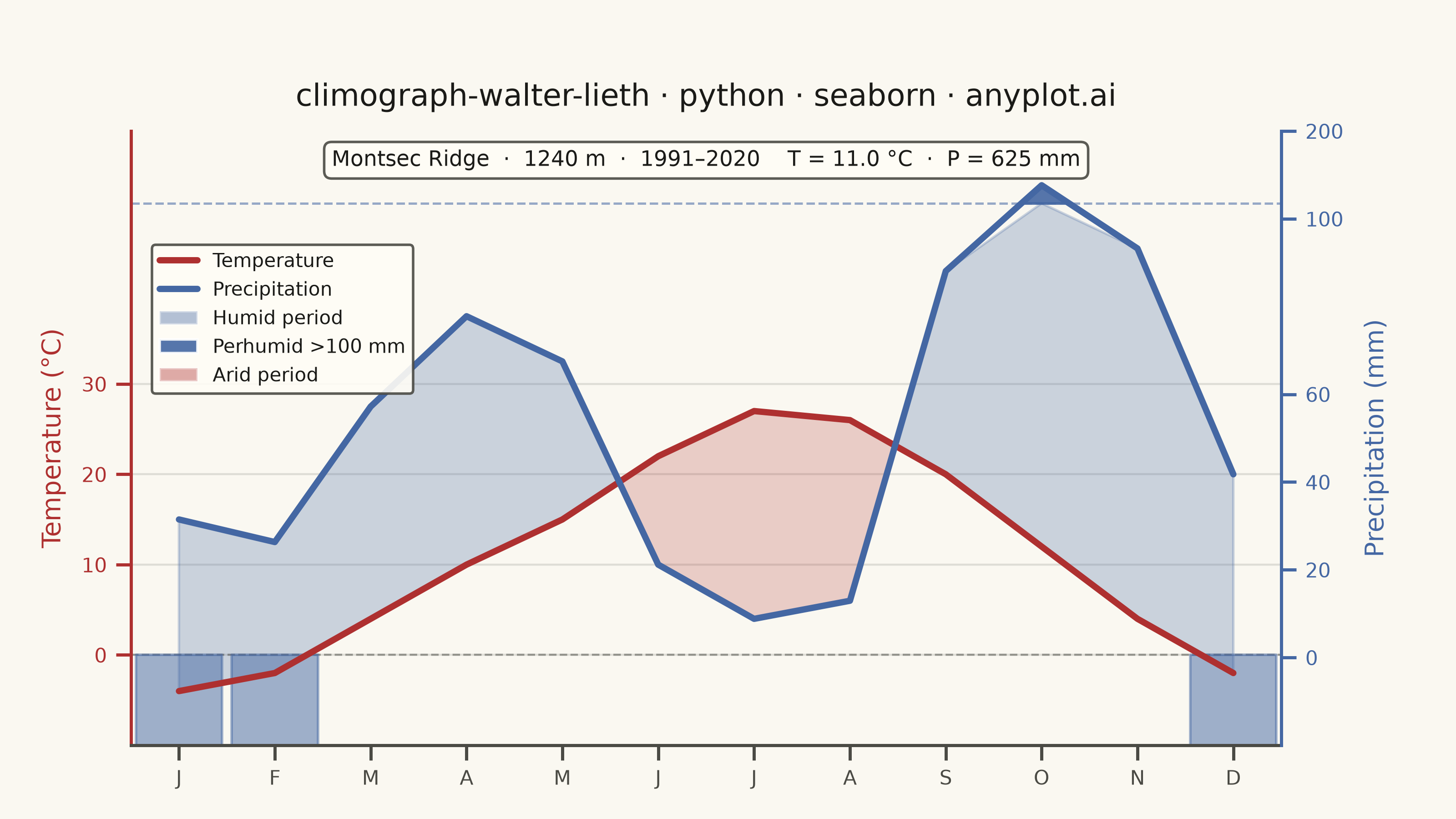
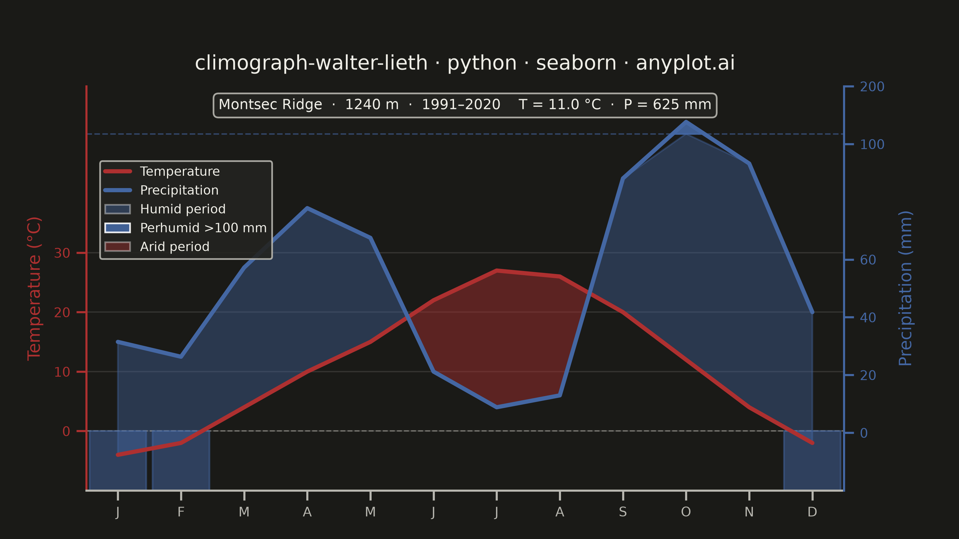
A Walter-Lieth climate diagram (climograph) is the canonical visualization of a location's annual climate, plotting monthly mean temperature and monthly precipitation over the twelve months on a single panel. It uses the classic 1:2 axis-scaling convention where 10 °C on the temperature axis aligns with 20 mm on the precipitation axis, so the relationship between the two curves directly reveals water availability: where precipitation exceeds the temperature curve the period is humid (filled blue/hatched), and where the temperature curve rises above precipitation the period is arid (filled red/dotted). A header carries station metadata and annual means, while frost indicators along the baseline mark cold months.
""" anyplot.ai
climograph-walter-lieth: Walter-Lieth Climate Diagram
Library: seaborn 0.13.2 | Python 3.13.13
Quality: 88/100 | Created: 2026-06-15
"""

import os
import sys


# Prevent the script directory from shadowing the seaborn package on sys.path
_this_dir = os.path.abspath(os.path.dirname(__file__))
sys.path = [p for p in sys.path if os.path.abspath(p) != _this_dir]

import matplotlib.lines as mlines
import matplotlib.patches as mpatches
import matplotlib.pyplot as plt
import numpy as np
import seaborn as sns


# Theme tokens
THEME = os.getenv("ANYPLOT_THEME", "light")
PAGE_BG = "#FAF8F1" if THEME == "light" else "#1A1A17"
ELEVATED_BG = "#FFFDF6" if THEME == "light" else "#242420"
INK = "#1A1A17" if THEME == "light" else "#F0EFE8"
INK_SOFT = "#4A4A44" if THEME == "light" else "#B8B7B0"

# Imprint palette — semantic assignments
# Temperature → matte red (Imprint slot 5, semantic: heat)
# Precipitation → blue (Imprint slot 3, semantic: water/sky)
TEMP_COLOR = "#AE3030"
PRECIP_COLOR = "#4467A3"

sns.set_theme(
    style="ticks",
    rc={
        "figure.facecolor": PAGE_BG,
        "axes.facecolor": PAGE_BG,
        "axes.edgecolor": INK_SOFT,
        "axes.labelcolor": INK,
        "text.color": INK,
        "xtick.color": INK_SOFT,
        "ytick.color": INK_SOFT,
        "grid.color": INK,
        "grid.alpha": 0.15,
        "legend.facecolor": ELEVATED_BG,
        "legend.edgecolor": INK_SOFT,
    },
)

# Station: Pyrenean highland — demonstrates all Walter-Lieth features:
# frost months (Jan/Feb/Dec), summer arid period (Jun/Jul/Aug), perhumid autumn (Oct)
STATION = "Montsec Ridge"
ELEVATION = 1240
PERIOD = "1991–2020"

MONTHS = ["J", "F", "M", "A", "M", "J", "J", "A", "S", "O", "N", "D"]
TEMPERATURE = np.array([-4.0, -2.0, 4.0, 10.0, 15.0, 22.0, 27.0, 26.0, 20.0, 12.0, 4.0, -2.0])
PRECIP = np.array([30, 25, 55, 75, 65, 20, 8, 12, 85, 120, 90, 40])

T_MEAN = round(TEMPERATURE.mean(), 1)
P_TOTAL = int(PRECIP.sum())

# Walter-Lieth dual-scale: 10°C = 20 mm below 100 mm (2:1); above 100 mm compressed 10:1
# P ≤ 100 mm → precip_t = P / 2
# P > 100 mm → precip_t = 50 + (P − 100) / 10
PERHUMID_THRESHOLD = 100.0
PERHUMID_Y = PERHUMID_THRESHOLD / 2.0  # = 50.0 on temp axis

precip_t = np.where(PRECIP <= PERHUMID_THRESHOLD, PRECIP / 2.0, PERHUMID_Y + (PRECIP - PERHUMID_THRESHOLD) / 10.0)
x = np.arange(12)

Y_MIN = -10
Y_MAX = max(TEMPERATURE.max(), precip_t.max()) + 6  # ~58

# Figure (landscape 3200×1800)
fig, ax = plt.subplots(figsize=(8, 4.5), dpi=400, facecolor=PAGE_BG)
ax.set_facecolor(PAGE_BG)

# Theme-adaptive fill alphas: arid fill is nearly invisible on dark near-black surface
ARID_ALPHA = 0.45 if THEME == "dark" else 0.22
HUMID_ALPHA = 0.40 if THEME == "dark" else 0.26

# Humid fill (blue): where precip_t >= temperature, capped at perhumid threshold
ax.fill_between(
    x,
    TEMPERATURE,
    np.minimum(precip_t, PERHUMID_Y),
    where=precip_t >= TEMPERATURE,
    color=PRECIP_COLOR,
    alpha=HUMID_ALPHA,
    interpolate=True,
    zorder=1,
)

# Perhumid fill (solid blue): P > 100 mm — solid to mark "very wet" zone above 100 mm
perhumid_mask = PRECIP > PERHUMID_THRESHOLD
ax.fill_between(
    x, PERHUMID_Y, precip_t, where=perhumid_mask, color=PRECIP_COLOR, alpha=0.90, interpolate=True, zorder=1
)

# Arid fill (red): where temperature exceeds precipitation curve
ax.fill_between(
    x,
    TEMPERATURE,
    precip_t,
    where=TEMPERATURE >= precip_t,
    color=TEMP_COLOR,
    alpha=ARID_ALPHA,
    interpolate=True,
    zorder=1,
)

# Frost month indicators: solid blue bar from Y_MIN to 0 for months with mean T < 0°C
for i, t in enumerate(TEMPERATURE):
    if t < 0:
        ax.fill_between([i - 0.45, i + 0.45], [Y_MIN, Y_MIN], [0, 0], color=PRECIP_COLOR, alpha=0.50, zorder=2)

# Temperature and precipitation lines via seaborn
sns.lineplot(x=x, y=TEMPERATURE, ax=ax, color=TEMP_COLOR, linewidth=2.5, zorder=3)
sns.lineplot(x=x, y=precip_t, ax=ax, color=PRECIP_COLOR, linewidth=2.5, zorder=3)

# Perhumid threshold line — marks scale change at 100 mm
ax.axhline(PERHUMID_Y, color=PRECIP_COLOR, linewidth=0.9, linestyle="--", alpha=0.55, zorder=2)

# Zero-degree reference line
ax.axhline(0, color=INK_SOFT, linewidth=0.8, linestyle="--", alpha=0.5, zorder=1)

# Left (temperature) axis styling
ax.set_ylim(Y_MIN, Y_MAX)
ax.set_xlim(-0.5, 11.5)
ax.set_xticks(x)
ax.set_xticklabels(MONTHS, fontsize=8)
ax.set_yticks([0, 10, 20, 30])
ax.tick_params(axis="y", colors=TEMP_COLOR, labelsize=8)
ax.set_ylabel("Temperature (°C)", fontsize=10, color=TEMP_COLOR, labelpad=6)
ax.spines["left"].set_color(TEMP_COLOR)
ax.spines["bottom"].set_color(INK_SOFT)
ax.yaxis.grid(True, alpha=0.12, linewidth=0.8, color=INK, zorder=0)

# Remove top and right spines — seaborn-idiomatic
sns.despine(ax=ax, right=True, top=True)

# Right precipitation axis with dual-scale tick labels (0, 20, 40, 60, 100, 200 mm)
ax2 = ax.twinx()
ax2.set_ylim(Y_MIN, Y_MAX)

tick_mm = np.array([0.0, 20.0, 40.0, 60.0, 100.0, 200.0])
tick_pos = np.where(tick_mm <= PERHUMID_THRESHOLD, tick_mm / 2.0, PERHUMID_Y + (tick_mm - PERHUMID_THRESHOLD) / 10.0)
ax2.set_yticks(tick_pos)
ax2.set_yticklabels([str(int(p)) for p in tick_mm])
ax2.tick_params(axis="y", labelsize=8, colors=PRECIP_COLOR)
ax2.set_ylabel("Precipitation (mm)", fontsize=10, color=PRECIP_COLOR, labelpad=8)
ax2.spines["right"].set_color(PRECIP_COLOR)
ax2.spines["top"].set_visible(False)
ax2.spines["bottom"].set_visible(False)
ax2.spines["left"].set_visible(False)

# Legend with proxy artists
leg = ax.legend(
    handles=[
        mlines.Line2D([], [], color=TEMP_COLOR, linewidth=2.5, label="Temperature"),
        mlines.Line2D([], [], color=PRECIP_COLOR, linewidth=2.5, label="Precipitation"),
        mpatches.Patch(facecolor=PRECIP_COLOR, alpha=0.40, label="Humid period"),
        mpatches.Patch(facecolor=PRECIP_COLOR, alpha=0.90, label="Perhumid >100 mm"),
        mpatches.Patch(facecolor=TEMP_COLOR, alpha=0.40, label="Arid period"),
    ],
    fontsize=7.5,
    loc="upper left",
    bbox_to_anchor=(0.01, 0.83),
    facecolor=ELEVATED_BG,
    edgecolor=INK_SOFT,
    framealpha=0.9,
)
for text in leg.get_texts():
    text.set_color(INK)

# Station header
header = f"{STATION}  ·  {ELEVATION} m  ·  {PERIOD}    T = {T_MEAN} °C  ·  P = {P_TOTAL} mm"
ax.text(
    0.5,
    0.97,
    header,
    transform=ax.transAxes,
    ha="center",
    va="top",
    fontsize=8.5,
    color=INK,
    bbox={"boxstyle": "round,pad=0.35", "facecolor": ELEVATED_BG, "edgecolor": INK_SOFT, "alpha": 0.9},
)

# Title
title = "climograph-walter-lieth · python · seaborn · anyplot.ai"
n = len(title)
ratio = 67 / n if n > 67 else 1.0
title_fontsize = max(8, round(12 * ratio))
ax.set_title(title, fontsize=title_fontsize, fontweight="medium", color=INK, pad=10)

# Layout and save
fig.subplots_adjust(left=0.09, right=0.88, bottom=0.09, top=0.84)
plt.savefig(f"plot-{THEME}.png", dpi=400, facecolor=PAGE_BG)
plt.close()
Runnable source as JSON, for any HTTP client: https://api.anyplot.ai/specs/climograph-walter-lieth/seaborn/code. Any spec id and library id listed in llms-full.txt fit the same URL shape; every URL below is complete and callable.
{
  "spec_id": "climograph-walter-lieth",
  "language": "python",
  "library": "seaborn",
  "page": "https://anyplot.ai/climograph-walter-lieth/python/seaborn",
  "hub": "https://anyplot.ai/climograph-walter-lieth",
  "code_json": "https://api.anyplot.ai/specs/climograph-walter-lieth/seaborn/code",
  "spec_json": "https://api.anyplot.ai/specs/climograph-walter-lieth",
  "render_light_png": "https://storage.googleapis.com/anyplot-images/plots/climograph-walter-lieth/python/seaborn/plot-light.png",
  "render_dark_png": "https://storage.googleapis.com/anyplot-images/plots/climograph-walter-lieth/python/seaborn/plot-dark.png",
  "quality_score": 88.0,
  "license": "MIT",
  "guide": "https://anyplot.ai/llms.txt"
}
Part of Walter-Lieth Climate Diagram on anyplot.ai.